MATH 1.4: Solving equations |
PPLATO @ | |||||
PPLATO / FLAP (Flexible Learning Approach To Physics) |
||||||
|
MATH 1.4: Solving equations
1 Opening items
1.1 Module introduction
1.2 Fast track questions
1.3 Ready to study?
2 Solving linear equations
2.1 Simple linear equations
2.2 Equations linear in a function of x
2.3 Simultaneous linear equations
2.4 Graphical solutions
3 Solving quadratic equations
3.1 The solutions as zeros of a quadratic function
3.2 Sums and products of roots: factorizing the quadratic
3.3 The quadratic equation formula: completing the square
3.4 Roots for all equations: complex numbers
4 Solving more complicated equations
4.1 Solving polynomial equations
4.2 Graphical solutions
4.3 Numerical procedures
5 Closing items
5.1 Module summary
5.2 Achievements
5.3 Exit test
sketchSketch means draw a rough graph, showing the salient features – it does not mean plot the graph accurately.
The denominator is the number or expression on the bottom of a fraction.
distance = speed × time
You might have realized that we could have moved directly to Equation 3 by equating the total time T to the sum of the rest time tR and the total cycling time D/υ.
The numerator is the number or expression on the top of a fraction.
Always check that your answers satisfy the original equations and that they make sense.
This is not a linear equation in x.
Equations 5 and 6 each contain partial information about the problem; but we need all the information contained in both equations to solve the problem.
A fourth method of solving Equations 7 and 8 would have been to substitute for y in terms of x.
Try this for yourself by substituting for x (from one equation) in terms of y (in the other).
The right–hand side of Equation 16 is sometimes referred to as a quadratic expression or simply a quadratic.
Note the terminology; equations have roots (i.e. solutions) while functions have zeros.
The case a > 0 gives a ‘happy’ curve, and a < 0 gives a ‘sad’ curve. (‘Happy’ and ‘sad’ are not recognized mathematical terms!)
For example, a quadratic equation with roots 2 and −5, is
(x − 2)(x + 5) = 0
which expands to x2 + 3x − 10 = 0. Any constant multiple of this equation would also have roots 2 and −5.
The fact that there are very few choices of integers that multiply to give 6 helps us considerably in this case.
If (2x + 3)(x + 1) = 0 then either (2x + 3) = 0 or (x + 1) = 0. Thus the roots are x = −3/2 and x = −1.
In FLAP square roots are generally regarded as representing quantities that may be positive or negative, so strictly speaking the ± sign is superfluous. However, we are retaining it here and treating it as a reminder that a square root may be positive or negative.
This shows the value of remembering the relations between the roots and coefficients of a quadratic equation as well as the formula.
Some engineers, and physicists who work with complex numbers use j instead of i, but all mathematicians, and most physicists, use i.
Notice that the imaginary part of 3 + 5i is 5 not 5i.
In physics and engineering, complex numbers are invaluable in calculations involving electrical circuits, where the two parts can be associated with the oscillatory and decay properties of the circuits. They are also useful in the study of waves and optics, and in many other areas.
Note the general form
| result | |
| denominator | numerator |
The result on the top is worked out term by term starting with x2. We multiply the denominator by x2 to get x3 − x2. This is written below the numerator and subtracted from it, leaving −5x2 + 11x − 6. We then proceed to divide this by the dominator x − 1, thus finding that the second term in the result is −5x, and so on.
Some computer programs that perform algebraic manipulations will factorize expressions of this kind.
More accurately, the points of intersection are
| x = −2.0325 | y = 0.7128 |
| x = 0.0719 | y = 0.7336 |
| x = 1.7106 | y = −0.8369 |
(but these values were found by numerical, rather than graphical, methods).
This is a version of the two–point form of the equation of a straight line. See the Glossary for details.
You may wish to verify that
$x=\dfrac{2x^3-1}{3x^2-4}$
is a rearrangement of the equation
$x^3-4x+1=0$
Don’t worry about how we found this rearrangement – that is dealt with in another module under the heading Newton–Raphson formula (see the Glossary).
Notice that after three iterations the solution is consistent with the answer to Question T19 which was given to five decimal places.
1 Opening items
1.1 Module introduction
When we do anything in physics, there comes a point when we have to produce numbers; either as the result of an experimental measurement, or as the prediction of a theory, or both. Almost always this means having to do some calculations; not just adding numbers, or multiplying them, but manipulating them in some way so as to produce an answer; often this involves solving_the_equationsolving equations. In this module we will look at how to solve the simplest (and commonest) equations, and outline some of the more generally applicable ways in which we can solve more difficult problems.
Initially, we will look at solving linear equations (in Section 2), i.e. equations in which the independent variable appears only as the first power. In Section 3 the discussion is extended to the solution of quadratic equations by various methods, e.g. factorizing, completing the square and using the quadratic equation formula. Finally, in Section 4 graphical and numerical procedures for solving polynomial equations are described.
The first thing you must do before starting this module is to PUT YOUR CALCULATOR AWAY. You will not need it for most of this module, and you will be told when you do need it. Calculators are very useful for doing calculations to great accuracy, but they can stop you thinking about the important features of calculations; they are often a good means of making mistakes quickly!
Study comment Having read the introduction you may feel that you are already familiar with the material covered by this module and that you do not need to study it. If so, try the following Fast track questions. If not, proceed directly to the Subsection 1.3Ready to study? Subsection.
1.2 Fast track questions
Study comment Can you answer the following Fast track questions? If you answer the questions successfully you need only glance through the module before looking at the Subsection 5.1Module summary and the Subsection 5.2Achievements. If you are sure that you can meet each of these achievements, try the Subsection 5.3Exit test. If you have difficulty with only one or two of the questions you should follow the guidance given in the answers and read the relevant parts of the module. However, if you have difficulty with more than two of the Exit questions you are strongly advised to study the whole module.
Question F1
Find the value of x that satisfies the following equation:
$\dfrac{x-1}{x+1} = 2$
Answer F1
x = −3
Question F2
Solve the following equations:
x + 2y = 4, 2x − y = 3
Answer F2
x = 2, y = 1
Question F3
Find the roots of the following equation:
x2 + x − 1 = 0
leaving the square roots in the answer. How can you verify that your answers are right?
Answer F3
x = ½ (−1 ± 5 ). The sum of the roots is −1, and their product is also −1
(If you do not understand the previous sentence you should take this as an indication that you should read the module.)
1.3 Ready to study?
Study comment In order to study this module you will need to understand the following terms: constant, equation, function, graph, power_mathematicalpowers, square root and variable. If you are uncertain about any of these terms you should review them now by referring to the Glossary, which will indicate where in FLAP they are developed. In addition, you will need to be able to expand, simplify and evaluate simple algebraic expressions that involve brackets. You will also need to be able to sketch and plot the graphs of simple functions. If you are uncertain about your ability to perform these operations, you should again refer to the Glossary for further information. The following questions will help you to check that you have the required skills and knowledge before embarking on this module.
Question R1
Expand the following expressions:
(a) (a − 2b)(a + 2b) (b) (x + 3)(x − 4) (c) (p − 3)2
Answer R1
(a) a2 − 4b2 (b) x2 − x − 12 (c) p2 − 6p + 9.
Question R2
Simplify the following expression:
2 (x2 + 3x − 2) − (2x2 − 6x − 4)
Answer R2
12x
Question R3
Iff (x) = 3x + 2, write down expressions for f (2y) and f (y − 1).
Answer R3
f (2y) = 3 (2y) + 2 = 6y + 2, f (y − 1) = 3 (y − 1) + 2 = 3y − 1
Question R4
What are the square roots of x4?
Answer R4
+x2 and −x2
Question R5
Sketch i graphs of the following functions from x = −1 to x = 3:
f (x) = 2x − 1 and g (x) = x2 − 3x + 2
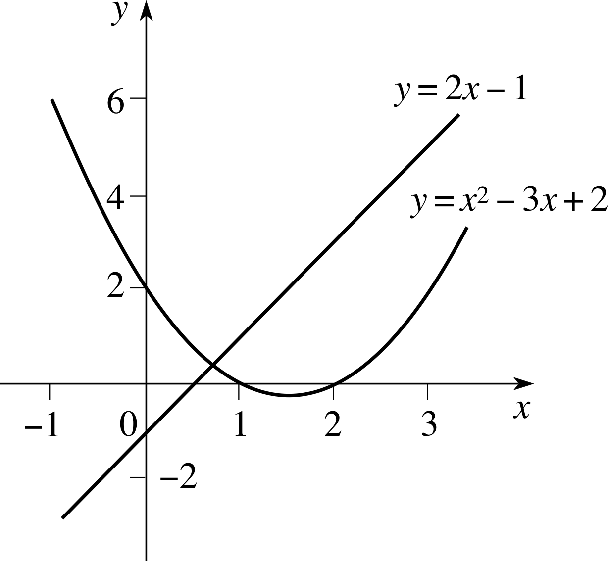
Figure 6 See Answer R5.
Answer R5
The graphs of the two functions are given in Figure 6.
Question R6
Rewrite, with a single denominator i, the expression:
$\dfrac{1}{x-1}-\dfrac{1}{x+1}$
Answer R6
$\dfrac{1}{1-x} - \dfrac{1}{1+x} = \dfrac{(1+x)-(1-x)}{(1-x)(1+x)} = \dfrac{2x}{1-x^2}$
2 Solving linear equations
When we attempt to solve an equation for an unknown variable, x say, we aim to find an expression which looks something like this
x = ???(1)
where the right–hand side does not involve x and is something we can calculate immediately. When we have reached this point the mathematics is done and arithmetic takes over.
In this section we shall look at linear equations, which only involve the first power of the unknown variable, x, rather than x2 or any higher power. In other words we will look at equations such as
3x + 2 = 5x − 2
which are said to be in linear form. We shall attempt to find the value (or values) of the unknown variable for which the equation is true. In the case of the above equation it is easy to see that the value x = 2 makes the equation true since for this value the left–hand side becomes 3 × 2 + 2 = 8, while the right–hand side is 5 × 2 − 2 = 8. We call this process solving the equation, and we speak of finding the solution, or finding the root of the equation. Later we will extend these notions to more than one equation. Equations that can be solved are sometimes said to be soluble, while those that can’t are insoluble.
2.1 Simple linear equations; solving by rearrangement
Suppose you set your stop–watch to zero as you start cycling along a road at 10 mph. After you have travelled 15 miles you stop for a rest. How long has this taken you?
The distance you have travelled after a period of time t is
d = υt i
where υ is your speed. In this example we know what d and υ are, and we have to find t. Dividing both sides of the above equation by υ we see that
$t = \dfrac{d}{\upsilon} = \dfrac{15}{10}\,{\rm hours}$
Thus we have reached the point at which arithmetic takes over and the final answer is 1.5 hours. This simple problem was solved by rearranging the equation.
Now for a slightly more complicated problem. Forget for the moment that d = 15 miles and υ = 10 mph, and think about the following problem in purely algebraic terms. Suppose that having cycled a distance d at speed υ you then rested for a time tR, and that following your rest you set out again on a second ride at speed υ. If you kept cycling until your total journey time (including the rest) was T, what distance would you have covered in that time?
The time spent on the second ride is found by subtracting the rest time and the time of the first ride from the total journey time, so it is (T − d/υ − tR); and the total distance D covered in both rides is just the sum of the distances covered in each ride, so
D = d + υ (T − d/υ − tR)(2)
It is easy to rearrange this equation to find an expression for T in terms of the total distance travelled, the speed, the distance d and the rest time. The form of this expression may already be obvious to you, but being systematic and spelling everything out in detail we can start by trying to isolate the bracket that contains T. To do this note that from Equation 2,
D − d = υ (T − d/υ − tR)
so that (T − d/υ − tR) = (D − d)/υ
Thus, T = d/υ + tR + (D − d)/υ = d/υ + tR + D/υ − d/υ
You can see that d/υ cancels out on the right–hand side of the last equation, so
T = tR + D/υ(3) i
Now we can substitute in some numbers; suppose the total distance travelled is 35 miles and υ = 15 mph; if the rest time was half an hour then tR = 0.5 hours and
$T = \rm \left(\dfrac12 + \dfrac{35}{10}\right)\,hours = (0.5 + 3.5)\,hours = 4\,hours$
You may be wondering why we didn’t put these numbers in at the beginning. There are three reasons for this; first, if you look again at Equation 3 you will see that the variable d has disappeared,
T = tR + D/υ(Eqn 3)
so less calculation is needed than if we had used numbers all the way through. Second, having worked out the general equation, we can change the distances, or the speed, and still find the time taken without having to go through the whole calculation again. Finally, it is often easier to check a calculation that involves algebraic variables rather than numerical values.
✦ Suppose you cycled non–stop for 36 miles at 12 mph. How long would this have taken?
✧ We just need to substitute tR = 0, D = 36 miles, υ = 12 mph in Equation 3 to obtain
T = (0 + 36/12) hours = 3 hours
This example provides us with a rule that applies throughout mathematics and physics. To avoid unnecessary effort and to reduce the chance of mistakes:
Don’t introduce numbers until it is essential; leave all the arithmetic until the end.
Let us now return to the business of solving equations. The following method applies to any equation in which the unknown variable appears to the first power only, and only in the numerator. i The procedure in general is much like the one described above; for brevity let us suppose the unknown variable is x.
To solve a linear equation, e.g. 3 (x − 1) = 2x + 5 (2 − x):
| (a) | if x appears in more than one bracket, expand the brackets; | 3x − 3 = 2x + 10 − 5x | |
| (b) | collect together all the terms involving x on one side of the equation and the remaining terms on the other; |
3x + 5x − 2x = 10 + 3 | |
| (c) | combine the coefficients of x as far as possible (i.e. simplify all the terms multiplying x), and then simplify all the remaining terms; |
6x = 13 | |
| (d) | you should now have an equation that can be written in the form of Equation 1 with no more than one more step. |
x = 13/6 |
With practice it is possible to condense this process by combining the steps, but be warned, doing too many steps in your head is likely to lead to mistakes. i Try the next four questions, all of which can be solved by the above method.
Question T1
Solve the equation:
2 (x + 1) = x − 5
Answer T1
2 (x + 1) = x − 5
This is equivalent to 2x + 2 = x − 5, therefore 2x − x = −5 − 2 and x = −7
To check this solution, substitute the value for x in the equation:
left–hand side = 2 (−7 + 1) = −12, right–hand side = −7 − 5 = −12
Question T2
Solve the equation:
(z − 2) + 3 (2z + 1) − (5z − 7) = 0
Answer T2
z − 2 + 6z + 3 − 5z + 7 = 0
If the terms are collected, z + 6z − 5z − 2 + 3 + 7 = 0, 2z + 8 = 0, so z = −4
To check this solution, substitute the value for x in the equation:
−6 + 3 (−7) − (−20 − 7) = −6 − 21 + 27 = 0.
Question T3
If a = 1 and b = 4, find the value of p that satisfies:
p − a = 3p + 2b
Answer T3
In terms of a and b the solution for p is p = −½ (a + 2b)
Now if we substitute for a and b, we obtain p = −½ (1 + 8) = −9/2
Question T4
If a = 4 and b = −2, find the value of p that satisfies:
p − a = 3p + 2b
Answer T4
Notice that we do not need to solve the equation again. We simply substitute the new values for a and b in the equation found in Answer T3, therefore, p = ½ (4 − 4) = 0
It is sometimes possible to solve what appear to be more complicated problems in the way described above. The general principle is to reduce more complicated equations to a form that we know how to solve. For example,
$\dfrac{x-1}{x+2}=3$(4)
can be rewritten, if both sides are multiplied by (x + 2), as
x − 1 = 3 (x + 2)
and then treated as before. However, it is not always possible to reduce such an equation to linear form.
✦ Try to simplify the following:
$\dfrac{x-1}{x+2}=\dfrac 3x$
✧ If we multiply by (x + 2) and by x, to obtain
x (x − 1) = 3 (x + 2) i
we are left with a term in x2, which cannot be removed. We shall see later that such equations can be solved, but for the moment we stop here.
There are many equations that appear at first sight to be beyond the realm of linear equations, but which can be simplified to an unexpected degree. Look, for example, at the following
$\dfrac{x-1}{x+2} = \dfrac{x+3}{x-1}$
If we multiply both sides of the equation by (x + 2)(x − 1) we have
(x − 1)2 = (x + 3)(x + 2)
which implies
x2 − 2x + 1 = x2 + 5x + 6
i.e.7x = −5
sox = −5/7
However, events like this should be regarded as just a lucky accident, and are not to be relied on – though it is legitimate to hope!
Question T5
Which of the following equations can be reduced to a linear form? Solve those which can.
(a) $\dfrac{1}{x-1}=6$ (b) $x^2-1=\dfrac{2}{x+1}$ (c) $x^2+2=x(x-3)$ (d) $\dfrac{(x+2)(x-2)}{x^2-4}=x$
Answer T5
(a) $\dfrac{1}{x-1} = 6$, so 1 = 6 (x − 1) or 6x = 7 and therefore x = 7/6
(b) There is no cancellation here; multiplying both sides by (x + 1) gives (x + 1)(x2 − 1) = 2 which expands to give x2 + x2 − x − 1 = 2, so this equation cannot be reduced to linear form.
(c) If we expand the bracket, x2 + 2 = x2 − 3x, so 2 = −3x or x = −2/3.
(d) If we expand the left–hand side we get $\dfrac{x^2-4}{x^2-4}=x$, which gives (after cancellation) x = 1
In real life it is not always obvious (as we can see from what we have just discussed) which equations can be reduced to the form of Equation 1. There is no general method which will allow us to take an arbitrary equation and say ‘yes, this can be solved like this’, and then write down the answer. Some equations can be solved easily, some with more difficulty, and some are impossible to solve. One of the advantages that comes from practice is the ability to recognize the category to which a particular equation belongs, so that you don’t waste time trying to solve something insoluble, and you can go straight to the right method for something soluble.
2.2 Equations linear in a function of x
There is a slight and fairly obvious generalization of the linear equation that arises if the variable is, say x2, rather than x. For example,
x2 + 4 = 2x2 − 12
can be solved for the unknown variable x2 to give x2 = 16, i.e. x = ±4. A similar method can be used in the following example.
✦ Solve the following equation:
1/(x − 1) + 2 = 2/(x − 1) − 4
✧ In this case we initially solve for the unknown variable 1/(x − 1).
Thus 1/(x − 1) − 2/(x − 1) = −4 − 2
so 1/(x − 1) = 6
We then solve this equation for x, as in Question T5(a), to obtain
x = 7/6
We could have reduced the chance of a mistake in copying, by substituting y = 1/(x − 1) at the start of this question. This trick is well worth remembering – try it on the next exercise.
Question T6
Solve the following equation:
$ 2\left(\dfrac{x^2+1}{x^2-1}+1\right) = \dfrac{x^2+1}{x^2-1}+5 \quad\left(\text{hint: put }y = \dfrac{x^2+1}{x^2-1}\right)$
Answer T6
If we put
$y = \dfrac{x^2+1}{x^2-1}$
then 2 (y + 1) = y + 5, 2y + 2 = y + 5, so y = 3
If we then substitute for y, we have
$\dfrac{x^2+1}{x^2-1} = 3,~~~x^2+1 = 3(x^2-1),~~~2x^2 = 4,~~~x^2 = 4$
so$x = \pm\sqrt{2\os}$. If we put $x = +\sqrt{2\os}$ in the original equation to check this, we find
the left–hand side is $2\left(\dfrac{2+1}{2-1}+1\right) = 8$ and the right–hand side is $2\left(\dfrac{2+1}{2-1}+5\right) = 8$
This can then be repeated for $x = -\sqrt{2\os}$
2.3 Simultaneous linear equations
Let us reconsider the cycling problem discussed in Subsection 2.1. Again suppose that you cycled along a road at a steady 10 mph. One hour after you left, a friend set off in a car at a steady 30 mph to catch you up. Where and when will you meet?
Let us take the distance to the meeting–point to be dm, and the time on your stop–watch to be tm when you meet. To keep things as general as possible, take the time at which the car starts to be T0, and the speeds of the bicycle and the car to be υ and V, respectively. At the instant you meet you will each have travelled the same distance, and so we have two equations analogous to Equation 2:
distance travelled by you = your speed × time spent cycling
i.e.dm = υtm(5)
and
distance travelled by your friend = your friend’s speed × time spent driving
i.e.dm = V (tm−T0)
sodm = Vtm− VT0(6)
We know the values of υ and V in these equations, and we can calculate VT0; but we do not know the distance dm or the time tm, and we cannot work them out from either Equation 5 (dm = υtm) or Equation 6 (dm = Vtm − VT0 ) alone. i Equations 5 and 6 are called simultaneous linear equations since they must be solved together if they are to be solved at all.
The basic method of solving a pair of equations of this kind involves substitution. This means that we find an expression for one of the variables using one equation, and we then substitute that expression for the selected variable in the other equation. For instance, Equation 5 tells us that we can replace dm by υtm; making this substitution in Equation 6 gives
υtm = Vtm − VT0
i.e.υtm −Vtm = −VT0
i.e.(υ − V)tm = −VT0
so$t_{\rm m} = \dfrac{-VT_0}{\upsilon-V} = \dfrac{VT_0}{V-\upsilon}$
This is part of the solution we seek since it expresses one of the unknown quantities (tm) in terms of known quantities. (It also makes good sense physically. Notice that tm increases as T0 increases, which we should expect, because the later your friend leaves, the longer it will be before you meet. Furthermore, if V = υ the bicycle and the car are travelling at the same speed, so the denominator becomes zero, tm becomes infinite, and you never meet – which is again what we expect.) All that remains now is to find dm, which we can do directly by substituting for tm in Equation 5:
dm = υVT0/(V − υ)
Now we can put in the numerical values υ = 10 mph, V = 30 mph, T0 = 11 h, and find
tm = $\left(\dfrac{30\times 1}{30-10}\right)$ hours = 1.5 hours and dm = (10 × 1.5) miles = 15 miles
Finally, we should check to see that these values do actually satisfy the original equations. We have used Equation 5 directly to find dm, but Equation 6 correctly gives
15 miles = 30 mph × (1.5 − 1) h = 15 miles
You will have noticed that we have put great emphasis on checking the answers; many wrong answers are due to bad arithmetic and algebraic slips. Always check that your answers satisfy the original equations and that they make sense. For example, an answer tm = −3 hours would not be sensible.
Notice that the problem we have just solved had two equations and two unknown variables tm and dm. In general, a pair of simultaneous linear equations may look more like this:
x + 2y = 8(7)
2x − 3y = −5(8)
and we may be required to solve these equations for the two variables x and y.
We can express x in terms of y (using Equation 7)
x = −2y + 8(9)
and then substitute for x in Equation 8 to obtain
2 (−2y + 8) − 3y = −5
so that−14y + 16 − 3y = −5
i.e.7y = 21
givingy = 3
If we substitute this value for y in Equation 9,
x = −2y + 8(Eqn 9)
we obtain
x = (−2 × 3) + 8 = 2
Now we should check to see that these answers satisfy the original equations. We have just used Equation 7 (in the form of Equation 9) to find x, so we check by substituting both values into the other equation, Equation 8,
2x − 3y = −5(Eqn 8)
and we find
(2 × 2) − (3 × 3) = 4 − 9 = −5
which is correct.
Notice that for checking we always use the original equation (before we have had a chance to make any mistake), and we don’t use the equation that has just been used to find one of the variables.
You can apply this same procedure to any pair of linear equations. However, if the coefficients are not the simple integers we have here, the algebra may soon start to look complicated, and it is useful to have some sort of drill for the process of solution. Look again at the equations we have just solved.
x + 2y = 8(Eqn 7)
2x − 3y = −5(Eqn 8)
To get an equation involving just y, multiply the equations by suitable factors so that both have the same coefficient of x – in this case we multiply both sides of Equation 7 by 2 and leave Equation 8 unchanged:
2x + 4y = 16
2x − 3y = −5(Eqn 8)
Now subtract the second equation from the first, to get
(2x + 4y) − (2x − 3y) = 16 − (−5)
i.e.0x + 7y = 21
so, as before, y = 3
This process is called elimination, we speak of eliminating x from the equations, though it’s really just a systematic way of implementing substitution.
We now proceed as before and use Equation 7 to give x = 2 again. After this we should use Equation 8 to carry out the same check.
Alternatively, we could have eliminated y from Equations 7 and 8; and the simplest way to do that is to multiply Equation 7 by 3, and Equation 8 by 2 to obtain
3x + 6y = 24
4x − 6y = −10
Now we may add the above equations to obtain
7x + 0y = 14
which gives x = 2
We can then use either Equation 7 or Equation 8 to find y, and the other to check the answer.
So we have seen three alternative methods of solving Equations 7 and 8:
- substituting for x (found from one equation) in terms of y (in the other)
- eliminating x
- eliminating y.
i In general we try to choose the method that is most convenient.
Question T7
Solve the following pairs of equations:
(a) 5x + 2y = 0
(a) 2x + 5y = 21
(b) 4x + y = 10
(b) 3x − 2y = 1
Answer T7
(a) Multiply the first equation by 2 and the second by 5:
10x + 4y = 0
10x + 25y = 105
Subtract the first equation from the second: 21y = 105, so y = 5
Substituting this value in either equation gives x = −2. You can then use the other one to check the answer.
(b) Multiply the first equation by 2:
8x + 2y = 20
3x − 2y = 13
This time add the two equations: 11x = 33, so x = 3. Substituting this value in either equation gives y = −2
Did you remember to check the solution?
We can also work out the general solution to a pair of simultaneous equations using symbols rather than
numbers. For example, for the pair of equations i
ax + by = p(10)
cx + dy = q(11)
the solution (provided ad − bc ≠ 0) is
x = (dp − bq)/D(12)
y = (aq − cp)/D(13)
whereD = ad − bc(14)
This general solution is not particularly helpful, and certainly not worth remembering. However, you may meet it again when you study the theory of sets of three or more simultaneous equations.
Question T8
Show that Equations 12–14 provide the correct solution to Equations 7 and 8.
Answer T8
We have a = 1, b = 2, c = 2 and d = −3, so that D = 1 × (−3) − (2 × 2) = −7.
Also p = 8 and q = −5 so that (from Equation 12)
x = (dp − bq)/D(Eqn 12)
$x = \dfrac{[(-3)\times 8]-[2 \times(-5)]}{-7} =2 $
and (from Equation 13)
y = (aq − cp)/D(Eqn 13)
$y = \dfrac{-5-(2 \times 8)}{-7} =3 $
As you can see, the amount of work using this general method is not significantly less than the previous methods. Hence our reluctance to use it.
Before leaving the subject of simultaneous linear equations it’s worth noting that such equations are not always soluble. Here are two situations where Equations 10 and 11 do not have a solution.
Case 1
This is the case in which the equations are not independent – i.e. one equation is a multiple of the other, so the second equation provides no new information; an example would be the pair of equations
x + 2y = 8
and2x + 4y = 16
If we try to eliminate x from these equations we shall just end up with 0 = 0, a statement which is true, but not much use.
Case 2
This is the case in which the equations are inconsistent – they cannot both be true at the same time. For example,
x + 2y = 8
and2x + 4y = 15
If we try to solve this pair of equations we shall find 1 = 0, which is neither useful nor true.
The first case occurs when we don’t have enough information to solve a problem, the second when some of the information is wrong or inconsistent. Note that in either case the general solution of Equations 12–14 does not apply since D = 0.
In this section we have been concerned with two linear equations, and two unknowns; however, there are many occasions when one has to deal with three or more unknowns. In general:
If there are n unknowns, then n consistent independent linear equations are needed to solve the equations for the unknowns.
If we are given more than n consistent linear equations, they cannot all be independent, so we are free to select n of them that are independent and use those to find the n unknowns. Finally, it should be noted that when seeking a set of three or more independent linear equations it is not enough to require that no equation should be a multiple of any other; rather we have to demand that none of the equations can be expressed as a sum of multiples of the others. It is actually fairly easy to determine whether or not a given set of equations satisfies this requirement, but it requires techniques beyond the scope of this module.
2.4 Graphical solutions
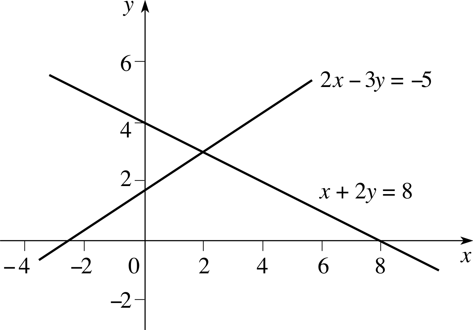
Figure 1 Graphical solution of Equations 7 and 8.
There is one other way of solving a pair of simultaneous equations that is worth mentioning – a graphical method. Let us consider Equations 7 and 8 yet again. If we write these in the equivalent form
$y=\dfrac{8-x}{2}$
$y=\dfrac{2x+5}{3}$
we can plot each of them as a straight–line graph, as in Figure 1. On the first line, y = (8 − x)/2, we have all the points (x, y) which make this equation a true statement. Similarly, on the second line, y = (2x + 5)/3, we have all the points (x, y) which make this equation a true statement. If both statements are true for a particular point (x, y) then this point must be where the two lines intersect, for it is only there that both equations are true simultaneously.
This method can be used to find an approximate solution to any pair of equations (linear or not) and it is often a good starting point, particularly if you have access to a graph–drawing computer or calculator.
Question T9
Use a graphical method to find approximate solutions of the simultaneous equations:
x + 2y = k and 2x − 3y = −5
for k = 2, 4, 6 and 8. (You can make use of Figure 1).
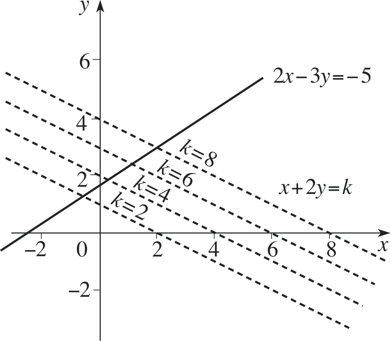
Figure 7 See Answer T9.
Answer T9
The intersection for various value of k is shown in Figure 7.
k = 2; x ≈ −0.6, y ≈ 1.3
k = 4; x ≈ 0.3, y ≈ 1.8
k = 6; x ≈ 1.1, y ≈ 2.4
k = 8; x ≈ 2.0, y ≈ 3.0
3 Solving quadratic equations
Up to now we have dealt with linear equations and their roots, that is, equations in which the independent variable appears only as the first power. Let us now advance to quadratic equations, which involve the square of the independent variable. The general form of a quadratic equation is
ax2 + bx + c = 0(15)
where a, b and c are constants. There is a simple general method of solving such equations which will be explained shortly, but it is instructive to examine the problem of solving quadratic equations from a number of other viewpoints, since it sheds a good deal of light on the general problem of solving equations.
3.1 The solutions as zeros of a quadratic function
A quadratic function is any function f (x) that may be written in the form
f (x) = ax2 + bx + c(16) i
where a, b and c are constants. Thus, when any given quadratic equation is written in the style of Equation 15, its left–hand side will define a corresponding quadratic function f (x). Moreover, it follows from Equations 15 and 16 that f (x) = 0 for each value of x that satisfies the given quadratic equation.
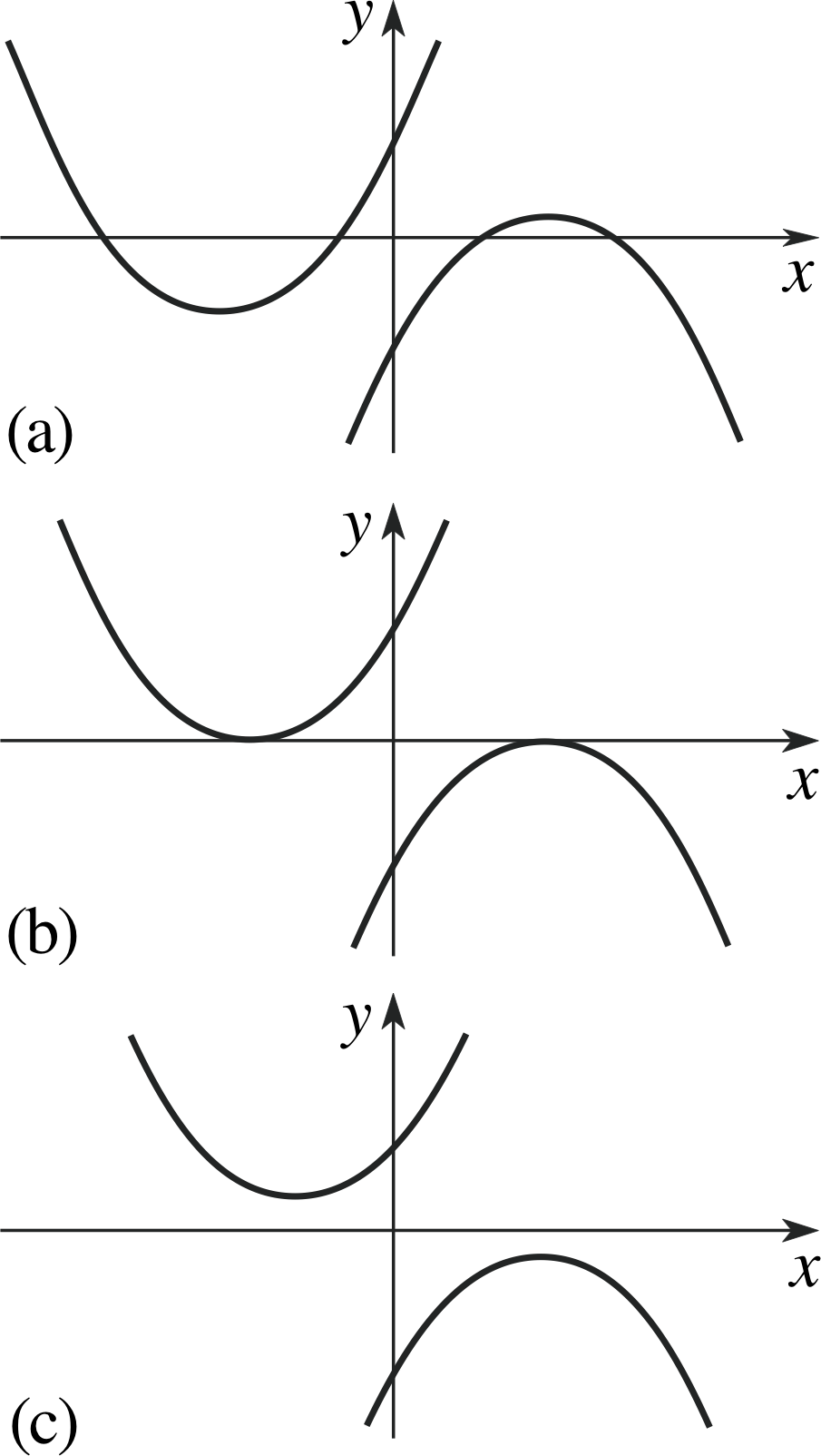
Figure 2 Graphs of six different quadratic functions.
For this reason the roots (or solutions) of a quadratic equation are also referred to as the zeros of the corresponding quadratic function. i
If we set y = f (x) and plot the graph of a quadratic function the resulting curve is called a parabola. Six different parabolas (corresponding to different values for a, b and c) are shown in Figure 2. If a > 0 the parabolas are as shown on the left of the figure, while the case a < 0 corresponds to those on the right. i
As you can see in Figure 2, the graph of any given quadratic function may meet the x–axis once or twice or not at all – it all depends on the values of a, b and c. However, if the graph does meet the x–axis it does so when y = f (x) = 0. It follows that each value of x at which the graph meets the x–axis is a zero of the quadratic function and therefore a solution (root) of the corresponding quadratic equation. The possibilities illustrated by the three parts of Figure 2 are as follows:
(a) there are two unequal roots, and the parabola crosses the x–axis in two distinct points;
(b) there is one root, at the point where the parabola just touches the x–axis;
(c) there are no roots, because the parabola never reaches the x–axis.
Case (b), where there is just one root, is really a special limiting case of (a).
If we move either of the parabolas in Figure 2a away from the x–axis its points of intersection with the x–axis (and hence the roots of the corresponding quadratic equation) will get closer and closer together, so that when the parabola just touches the x–axis, the two will have merged. For this reason we usually say that the root in (b) is a repeated root or that the equation has coincident roots.
These possibilities are the central feature of the process of solving quadratic equations, as we shall see.
3.2 Sums and products of roots: factorizing the quadratic
Throughout this section our aim is to solve the quadratic equation ax2 + bx + c = 0, by finding values for its roots, α and β say. But suppose for the moment that we know α and β and we ask instead ‘what is the quadratic equation that has α and β as its roots?’
An answer to this question is given by the equation
(x−α)(x−β) = 0(17)
It is easy to see that if we put either x = α or x = β in this equation then the left–hand side is zero (if α and β are equal, then we have a repeated root). Moreover, expanding the left–hand side of Equation 17 gives the quadratic equation
x2 − (α + β)x + αβ = 0(18)
In other words, the quadratic equation x2 − (α + β)x + αβ = 0 has α and β as its roots. i
Now, compare Equation 18 with the general quadratic equation we are trying to solve:
ax2 + bx + c = 0(Eqn 15)
We can make the general equation look more like Equation 18 by dividing both sides by a, which gives
x2 + (b/a)x + (c/a) = 0(19)
x2 − (α + β)x + αβ = 0(Eqn 18)
It then becomes clear that Equations 18 and 19 are the same, provided that
α + β = −b/a and αβ = c/a(20)
Thus, we can make the following connections between the coefficients of a quadratic and its roots.
Given a general quadratic equation ax2 + bx + c = 0 with roots α and β
- the sum of its roots is α + β = −b/a
- and the product of its roots is αβ = c/a (Eqn 20)
Unfortunately it is not possible to use these equations directly to solve the equation; if you try to do so you will just end up with the original equation! However, they may help us to factorize the original equation, that is to re–express it in the form of Equation 17 and hence identify its solutions. This is often the quickest method of solution, especially if we know, or suspect, that the roots are integers (i.e. whole numbers).
✦ Solve the equation:
x2 − 5x + 6 = 0
✧ In this case a = 1, b = −5 and c = 6, so we wish to find roots, α and β, such that α + β = 5 and αβ = 6. If the roots are integers then, apart from signs, they must either be 2 and 3, or 1 and 6, and both members of the pair must have the same sign, since their product is +6.
In this case only the values 2 and 3 meet all the requirements. i This means that the equation x2 − 5x + 6 = 0 can be written in the alternative form (x − 2)(x − 3) = 0, and now we can see that the roots are 2 and 3.
In the above solution we have used the process known as factorization to find the roots of the equation. We can check that our answer is correct by expanding the brackets to give
(x − 2)(x − 3) = x2 − 2x − 3x + 6 = x2 − 5x + 6
If we had to solve the almost identical equation
x2 − 5x − 6 = 0
we would have α + β = 5 and αβ = −6 and the roots would still involve 2 and 3, or 1 and 6, but this time the two numbers in each pair would have opposite signs, since the product αβ is negative. We must choose the pair + 6 and −1. We can check by expanding as before, and this time:
(x − 6)(x + 1) = x2 − 6x + x − 6 = x2 − 5x − 6
Question T10
Solve the following quadratic equations by factorization:
(a) x2 − 3x + 2 = 0
(b) x2 + x − 2 = 0
(c) x2 + 7x + 12 = 0
(d) x2 − x − 12 = 0
(e) x2 − 2x − 15 = 0
(f) x2 − 4x − 12 = 0
Answer T10
(a) (x − 1)(x − 2) = 0, so x = 1 or x = 2
(b) (x − 1)(x + 2) = 0, so x = 1 or x = −2
(c) (x + 3)(x + 4) = 0, so x = −3 or x = −4
(d) (x − 4)(x + 3) = 0, so x = 4 or x = −3
(e) (x − 5)(x + 3) = 0, so x = 5 or x = −3
(f) (x + 2)(x − 6) = 0, so x = −2 or x = 6
The above equations all had the coefficient of x2 equal to 1. It is a little more complicated if a is not 1. Consider, for example, the expression
2x2 + 5x + 3
If this can be factorized, then it must be possible to express it as
(2x + ?)(x + ?)
Trial and error shows us that the factorization is
(2x + 3)(x + 1)
Thus, to solve the equation 2x2 +5x+3 = 0 we rewrite it as (2x+3)(x+1) = 0 and then it is clear that the roots are −3/2 and −1. i
It is important to check your answer by substituting the values you have obtained back into the original equation to verify that they are indeed roots of the equation.
Question T11
Solve the following equations by factorization:
(a) 2x2 + 9x − 5 = 0
(b) 3x2 − 11x − 4 = 0
(c) 3x2 − x − 2 = 0
(d) 4x2 − 3x − 1 = 0
(e) 4x2 − 4x + 1 = 0
(f) 6x2 + 5x − 6 = 0
Answer T11
(a) (2x − 1)(x + 5), so x = 1/2 or x = −5
(b) (3x + 1)(x − 4) = 0, so x = −1/3 or x = 4
(c) (3x + 2)(x − 1) = 0, so x = −2/3 or x = 1
(d) (4x + 1)(x − 1) = 0, so x = −1/4 or x = 1
(e) (2x − 1)(2x − 1) = 0, so x = 1/2 (repeated root)
(f) (3x − 2)(2x + 3) = 0, so x = 2/3 or x = −3/2
With practice this method can become very quick, but unfortunately it does not always work. The quadratic equation
x2 − 3x + 1 = 0
cannot be factorized in the same way, because the roots are not integers. We must therefore find a more generally applicable method even if it is somewhat slower.
3.3 The quadratic equation formula: completing the square
The quadratic equation
x2 − 7 = 0
is easily solved, for we may simply add 7 to both sides of the equation and then take square roots of both sides to obtain
x2 = 7, so that $x = \pm\sqrt{7\os}$ i
The quadratic equation
(x + 3)2 − 5 = 0
is hardly more difficult, since we can add 5 to both sides, then take the square root of both sides to get
$x + 3 = \pm \sqrt{5\os}$ so that $x = -3 \pm \sqrt{5\os}$
If we could reduce the general quadratic equation to something like this form we should have another method of solution that might work more generally. Introducing such a method is the main purpose of this subsection, but first we must examine how one might write any quadratic equation in such a form. Another example may make the problem clear.
To solve the equation
3x2 − 10x + 1 = 0
we first extract the factor 3 to give
$3\left(x^2-\dfrac{10}{3}x+\dfrac13\right)=0$(21)
and we thus ensure that the coefficient of x2 inside the brackets is 1. Next we arrange for the term $x^2-\dfrac{10}{3}x$ to arise from a term of the form (x + k)2 for some value k. (Such a term is called a perfect square.)
Since (x + k)2 = x2 + 2kx + k2 we will be forced to choose k so that 2k = −10/3 in this case, in other words k = −5/3, which gives k2 = 25/9.
$3\left(x^2-\dfrac{10}{3}x+\dfrac13\right)=0$(Eqn 21)
Now we add and subtract 25/9 to the term in the brackets in Equation 21 to get
$3\left(x^2-\dfrac{10}{3}x+\dfrac{25}{9}-\dfrac{25}{9}+\dfrac13\right)=0$(22)
The advantage of this step is that the first three terms in the bracket can be written as a perfect square, so Equation 22 becomes
$3\left[\left(x^2-\dfrac53\right)^2-\dfrac{25}{9}+\dfrac13\right]=0$
and this can be simplified to
$3\left[\left(x^2-\dfrac53\right)^2-\dfrac{22}{9}\right]=0$
so that $\left(x^2-\dfrac53\right)^2=\dfrac{22}{9}$ and therefore $x = \dfrac53 \pm \dfrac{\sqrt{22\os}}{3}$
The above process is known as completing the square; try the same method in the following exercises.
Question T12
Find the roots of the following equations by completing the square:
(a) x2 − x − 2 = 0 (b) x2 − 2x − 8 = 0 (c) 2x2 + x − 10 = 0 (d) 3x2 − 18x + 24 = 0
Answer T12
(a) $x^2-x-2=x^2-x+\dfrac14 -\dfrac14-2=\left(x-\dfrac12\right)^2-\dfrac94$
hence $x-\dfrac12=\pm\sqrt{9/4\os}; x=\dfrac12\pm\dfrac32=2\;\text{or}\;-1$
(b) x2 − 2x − 8 = x2 − 2x + 1 − 1 − 8 = (x − 1)2 − 9
hence x − 1 = ± 9 ; x = 1 ± 3 = 4 or −2.
(c) $2x^2+x-10=2\left(x^2+\dfrac x2-5\right)=2\left(x^2+\dfrac x2+\dfrac{1}{16}-\dfrac{1}{16}-5\right)=2\left[\left(x+\dfrac14\right)^2-\dfrac{81}{16}\right]$
hence $\left(x+\dfrac14\right)^2=\dfrac{81}{16}; x+\dfrac14=\pm\dfrac94$; x = +2 or −2.5
(d) 3x2 − 18x + 24 = 3 (x2 −6x + 8) = 3 (x2−6x + 9 + 9 − 8) = 3 [(x −3)2 −1]
Hence (x − 3)2 − 1 = 0; x − 3 = ±1; x = 4 or 2.
To see how this method can be applied in general, let us repeat the procedure for the general quadratic.
$\begin{align}ax^2+bx+c & = a\left(x^2+\dfrac ba x+\dfrac ca\right) \\ & = a\left(x^2+\dfrac ba x+\dfrac{b^2}{4a^2}-\dfrac{b^2}{4a^2}+\dfrac ca\right) \\ & = a\left[\left(x+\dfrac{b}{2a}\right)^2-\dfrac{b^2-4ac}{4a^2}\right] \end{align}$
Now if we put this expression equal to zero, we can divide both sides by the multiplying factor a, and get
$\left(x+\dfrac{b}{2a}\right)^2-\dfrac{b^2-4ac}{4a^2} = 0$ so that $\left(x+\dfrac{b}{2a}\right)^2=\dfrac{b^2-4ac}{4a^2}$ and $x+\dfrac{b}{2a}=\pm\sqrt{\dfrac{b^2-4ac}{4a^2}}$
thus$x=\dfrac{-b\pm\sqrt{b^2-4ac}}{2a}$(23)
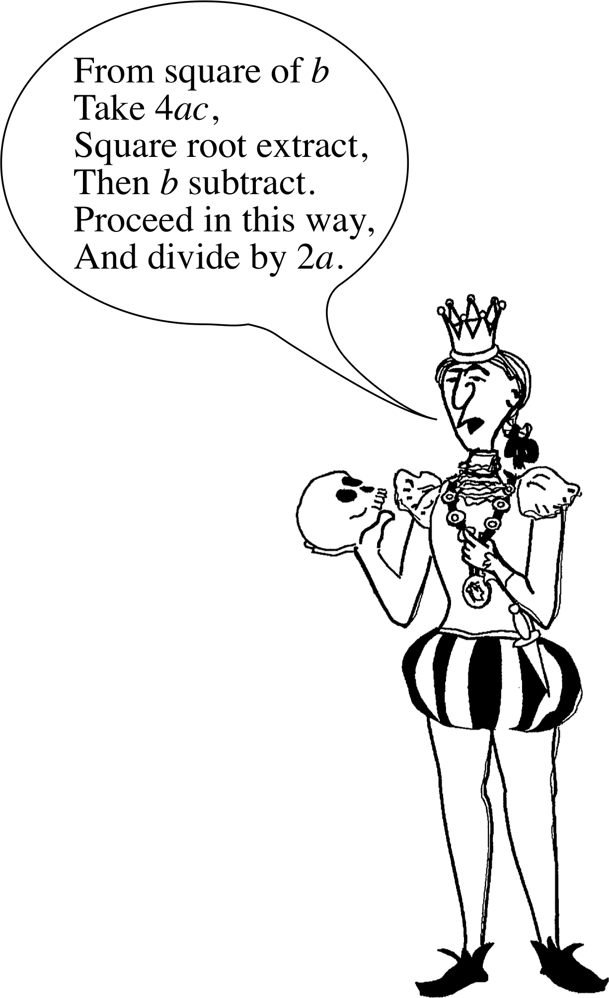
This is a very important formula, which is used so often that you should commit it to memory. (The author was taught a piece of doggerel i; you may, or may not, find it helpful.)
In practice this formula provides the simplest and quickest way of solving most quadratic equations.
Question T13
Use Equation 23 to solve the problems you met in Question T12; i.e find the roots of the following equations:
(a) x2 − x − 2 = 0 (b) x2 − 2x − 8 = 0 (c) 2x2 + x − 10 = 0 (d) 3x2 − 18x + 24 = 0
Answer T13
The answers are the same as those given in Answer T12:
(a) $x^2-x-2=x^2-x+\dfrac14 -\dfrac14-2=\left(x-\dfrac12\right)^2-\dfrac94$
hence $x-\dfrac12=\pm\sqrt{9/4\os}; x=\dfrac12\pm\dfrac32=2\;\text{or}\;-1$
(b) x2 − 2x − 8 = x2 − 2x + 1 − 1 − 8 = (x − 1)2 − 9
hence x − 1 = ± 9 ; x = 1 ± 3 = 4 or −2.
(c) $2x^2+x-10=2\left(x^2+\dfrac x2-5\right)=2\left(x^2+\dfrac x2+\dfrac{1}{16}-\dfrac{1}{16}-5\right)=2\left[\left(x+\dfrac14\right)^2-\dfrac{81}{16}\right]$
hence $\left(x+\dfrac14\right)^2=\dfrac{81}{16}; x+\dfrac14=\pm\dfrac94$; x = +2 or −2.5
(d) 3x2 − 18x + 24 = 3 (x2 −6x +8) = 3 (x2−6x + 9 + 9 − 8) = 3 [(x −3)2 −1]
Hence (x − 3)2 − 1 = 0; x − 3 = ±1; x = 4 or 2.
Question T14
Use Equation 23,
$x=\dfrac{-b\pm\sqrt{b^2-4ac}}{2a}$(Eqn 23)
to solve the following:
(a) x2 − 6x + 1 = 0 (b) 3x2 − 9x + 2 = 0
Do not use your calculator, but leave the answer in the simplest form possible, with the square roots not evaluated. Check that the sum and product of the roots are correct.
Answer T14
(a) $x = \dfrac12(6\pm\sqrt{36-4\os})=3\pm\sqrt{8\os}$
Sum of roots = $(3+\sqrt{8\os}) + (3-\sqrt{8\os}) = 6 = -b/a$; product of roots = $(3-\sqrt{8\os} )(3+\sqrt{8\os}) = 9 − 8 = 1 = c/a$.
(b) $x=\dfrac16(9\pm\sqrt{81-4\times 3\times 2\os}) = \dfrac16(9\pm\sqrt{57\os}$
Sum of roots = 3 = −b/a; product of roots = (1/36)(81 − 57) = 2/3 = c/a.
In both of these cases we use a2 − b2 = (a − b)(a + b) to find the product.
Figure 2 Graphs of six different quadratic functions.
Not only does Equation 23 simplify the process of solving quadratic equations, it also has a feature which enables us to say something about the general properties of the quadratic equation without actually having to solve it. This feature is known as the discriminant, and is given by the expression inside the square root, b2 − 4ac.
The sign of the discriminant determines some useful properties of the roots of the equation:
- If b2 − 4ac is positive, then we can find its square root, and the quadratic equation will have two different roots. This corresponds to the case (a) of Figure 2, where the parabola crosses the x–axis twice. (For reasons that will become clear in the next subsection, we also say that the equation has two distinct real roots.)
- If b2 − 4ac is equal to zero, then the two roots of the equation will be repeated and the quadratic equation can be written as a (x + k)2 = 0. This corresponds to the special case (b) of Figure 2 in which the parabola just touches the x–axis and we have just one (repeated) real root.
- If b2 − 4ac is negative, then we cannot take the square root, and we say that there are no real roots to the equation. This case corresponds to case (c) of Figure 2, when the parabola does not intersect the x–axis at all.
Question T15
Use the discriminant to establish how many real roots the following equations have:
(a) 4x2 − 20x + 25 = 0 (b) x2 + x + 6 = 0 (c) x2 + x − 6 = 0
Answer T15
(a) The discriminant = (−20)2 − 4 × 4 × 25 = 0; there are two equal roots.
(b) The discriminant = 1 − 4 × 6 = −23; there are no real roots.
(c) The discriminant = 1 − 4 × (−16) = 25; there are two real roots.
Although we now seem to have a recipe that will solve all our problems with quadratic equations, and make the whole business purely mechanical, this is not quite true. It often happens that when we have to substitute numbers in formulae, things are not quite as straightforward as appears at first sight. For example, consider the equation:
x2 − 2x + 10−12 = 0
and notice that the constant term, c, is very small.
If the constant term 10−12 were not there, the equation would be x2 − 2x = 0 which has roots at x = 2 and x = 0, so we would expect the given equation to have roots near these values.
Applying the formula (Equation 23) gives us the roots
$x = \left.\left(2 \pm \sqrt{4-4\times10^{-12}}\right)\middle/2\right.$
which can only be evaluated as 2 or 0 to the accuracy of most calculators.
The first root will certainly be as close to 2 as most people could wish, but to get the second root we have to take the difference of two numbers that are very close together, which means that we have lost a lot of precision. However, there is an alternative. If we calculate the larger root (say α) using Equation 23, we find a value near to 2 as before. We can then use the fact that the product of the roots (αβ) is equal to c/a, i.e. 10−12, to obtain the value 10−12/2 = 5 × 10⁻¹³ for the smaller root (say β). i
3.4 Roots for all equations: complex numbers
Let us look again at what happens when the discriminant b2 − 4ac is negative. Consider the equation
x2 − x + 1 = 0
for which a = 1, b = −1 and c = 1, so that b2 − 4ac = −3.
If we try to solve this equation using Equation 23,
$x=\dfrac{-b\pm\sqrt{b^2-4ac}}{2a}$(Eqn 23)
we get
$x = \dfrac12\left(1\pm\sqrt{-3\os}\right)$
which does not seem to make sense, since a negative number like −3 has no square root.
Yet if we substitute one of these ‘roots’ into the left–hand side of the equation we find:
$\begin{align}x^2-x+1 & = \left[\dfrac12\left(1-\sqrt{-3\os}\right)\right]^2-\dfrac12\left(1-\sqrt{-3\os}\right)+1 \\ & = \dfrac14\left[1-2\sqrt{-3\os}+\left(\sqrt{-3\os}\right)^2\right]-\dfrac12\left(1-\sqrt{-3\os}\right)+1 \\ & = \dfrac14\left(1-2\sqrt{-3\os}-3\right)-\dfrac12\left(1-\sqrt{-3\os}\right)+1 \\ & = -\dfrac12-\dfrac12\sqrt{-3\os}-\dfrac12\left(1-\sqrt{-3\os\os}\right)+1 = 0\end{align}$
So treating the quantity −3 as an ‘ordinary’ number such that its square is −3 appears to give us a solution to the equation.
Question T16
Show that:
$x=\dfrac12\left(1+\sqrt{-3\os}\right)$
also satisfies the equation x2 − x + 1 = 0 in the same way.
Answer T16
The proof is exactly the same as for $\dfrac12(1-\sqrt{-3\os})$, except that the sign in front of the square root is changed wherever the root appears.
Both ‘roots’ satisfy the equation, even if they do not mean anything! Since there seems to be no contradiction,
this is an invitation to mathematicians to invent something new.
A quantity called i is introduced, which is used in place of $\sqrt{-1\os}$ ; it has the property that i × i = −1. i This enables us to deal with the square root of any negative number; for example
$\sqrt{-3\os} = \sqrt{-1 \times 3\os} = \sqrt{-1\os} \times \sqrt{3\os} = i \sqrt{3\os}$
The number i can be given a perfectly sound mathematical definition, but that is not our concern here, we merely wish to use it. For example, we may write
i4 = (i2)2 = (−1)2 = 1
ori3 = i × i × i = −1 × i = −i
or$\dfrac1i = \dfrac{i}{i\times i} = \dfrac{i}{-1}= -i$
The quantity i and all its multiples, such as $i\sqrt{3\os}$, are examples of imaginary numbers. These should be contrasted with ‘ordinary numbers’ such as 35 or −2.6 that do not involve i and which are formally referred to as real numbers. By adding together real and imaginary numbers it is possible to create so–called complex numbers of the form
a + bi
where a and b are both real numbers. For example, 3 + 5i, would be a typical complex number.
The real number a is called the real part, and the real number b the imaginary part, of the complex number. The real part of 3 + 5i is 3 while its imaginary part is 5. i ‘Real’ and ‘imaginary’ are perhaps unfortunate names to have been chosen, since they suggest that a is more important than b, whereas we must treat both on an equal footing. However, the names are now too well established to be changed easily.
Question T17
Using complex numbers, find the solutions of the following equations:
(a) x2 + 25 = 0 (b) x2 + x + 6 = 0
Answer T17
(a) $x^2=25; x=\sqrt{-25\os}=\sqrt{25\times (-1)\os}=\sqrt{25\os}\times\sqrt{-1\os}=\pm5i$
(b) From Equation 23,
$x=\dfrac{-b\pm\sqrt{b^2-4ac}}{2a}$(Eqn 23)
$x=\dfrac12\left(-1\pm\sqrt{1-4\times 6\os}\right)=\dfrac12\left(=1\pm i\sqrt{23\os}\right)$
Complex numbers play an important part in mathematics and physics, and are the subject of a whole block of FLAP modules. i
We cannot go into all their applications here, but it is worth noting that if we allow roots to be complex, and if we count repeated roots twice, then every quadratic equation has two roots, the values of which are given by Equation 23.
$x=\dfrac{-b\pm\sqrt{b^2-4ac}}{2a}$(Eqn 23)
4 Solving more complicated equations
The equations we have dealt with so far are a very small sample of the variety that you will meet. We mentioned simultaneous equations with more than two unknown quantities in Subsection 2.3, but you will also meet equations that involve higher powers of the unknown variable than the square, including cubic equations such as
x3 + x2 + x + 1 = 0
and quartic equations such as
x4 + x3 + x2 + x + 1 = 0
Such equations, together with the linear and quadratic equations we considered earlier, are special cases of a class of polynomial equations which have the general form
a0 + a1x + a2x2 + ... + an−1x n−1 + anx n = 0
where n is an integer called the degree of the polynomial, and the n + 1 constants a0, a1, a2, ... an−1 and an are the coefficients of the polynomial. The left–hand side of such an equation constitutes a polynomial expression and may be used to define a corresponding polynomial function.
There is a general result for roots of polynomial equations:
The fundamental theorem of algebra states that every polynomial equation of degree n has precisely n roots as long as complex roots and repeated roots are counted.
Cubic and quartic equations can be solved using formulae similar to that used for solving quadratic equations, but these formulae are so complicated that they are rarely used. However, there are no general formulae for the roots of equations of the 5th and higher degrees, and in such cases we must usually be satisfied with numerical approximations. Many of the numerical methods that are used for finding these approximations can also be applied to non–polynomial equations and we shall examine such methods shortly. First, however, let us look at methods that allow us to solve some polynomial equations.
4.1 Solving polynomial equations
Sometimes, if we are fortunate, we are able to guess one, or more, solutions of a cubic, or higher order, equation and this makes the task of finding the remaining roots considerably easier. For example, if we substitute x = 1 into the left–hand side of the following equation:
x3 − 6x2 + 11x − 6 = 0(24)
we see immediately that this value of x makes the equation true. It follows that (x − 1) is a factor of the left–hand side of Equation 24 so that
x3 − 6x2 + 11x − 6 = (x − 1) × (a quadratic expression in x)
i.e.$\dfrac{x^3 - 6^2x + 11x - 6}{x-1}$ = a quadratic expression in x
We can find this quadratic expression by algebraic division as follows:
| x2 | − | 5x | + | 6 | i | ||
| x − 1 | x3 | − | 6x2 | + | 11x | − 6 | |
| x3 | − | x2 | |||||
| − | 5x2 | + | 11x | ||||
| − | 5x2 | + | 5x | ||||
| + | 6x | − 6 | |||||
| + | 6x | − 6 |
so that x3 − 6x2 + 11x − 6 = (x − 1)(x2 − 5x + 6).
The quadratic expression on the right is then easily factorized to give
x3 − 6x2 + 11x − 6 = (x − 1)(x − 2)(x − 3)
and now we can see that the roots of Equation 24 are 1, 2 and 3.
This method is quite restricted in its applications because it relies on our ability to guess a root, but it can still be very useful. i
Question T18
Find the roots of x3 + x2 − 4x − 4 = 0.
(Hint: try some integer values of x.)
Answer T18
One of your first trials should show that x = −1 is a solution. Then taking out the factor (x + 1) gives
x3 +x2 − 4x − 4 = (x +1)(x2 − 4)
x3 +x2 − 4x − 4 = (x + 1)(x − 2)(x + 2)
and the roots are therefore −1, 2 and −2.
4.2 Graphical solutions
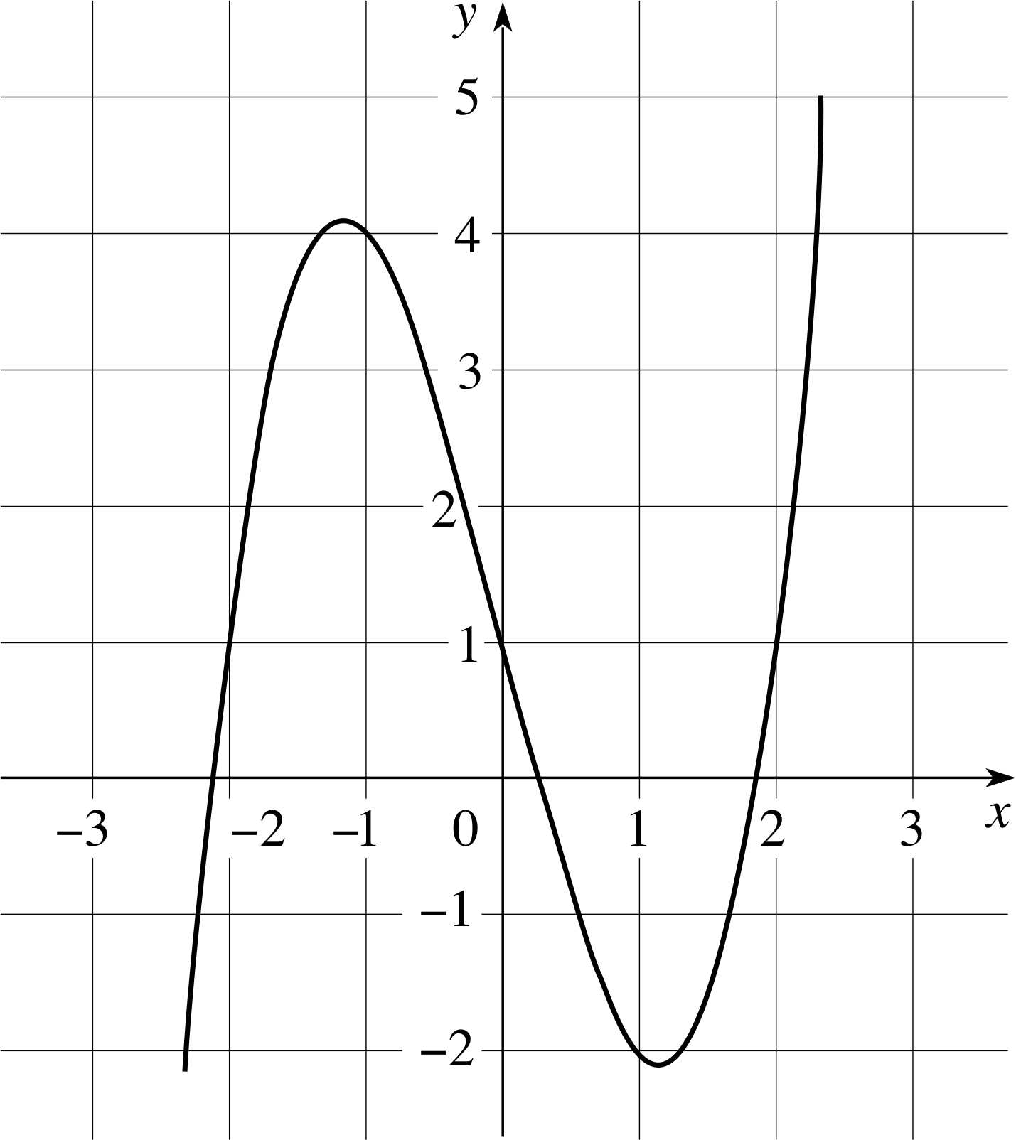
Figure 3 The graph of Equation 25.
In Subsection 2.4 we saw how we could use graphs to solve a pair of simultaneous equations, and in Section 3 we saw how a graph of a quadratic function could give us clues about the roots of the 4 corresponding quadratic equation. Similar methods can be applied to a wide variety of equations. Consider, for example, the function
f (x) = x3 − 4x + 1(25)
the graph of which is shown in Figure 3.
The curve crosses the x–axis three times, so the equation f (x) = 0 has three roots, which are, respectively, near −2, between 0 and 1, and near +2. A larger scale graph would tell us that the values are nearer −2.1, 0.25 and +1.9. If this degree of precision is enough, then nothing further need be done. If greater accuracy is needed, then one has the choice of drawing a yet more accurate graph (or perhaps three separate graphs, one for the neighbourhood of −2 each root) or of using another method.
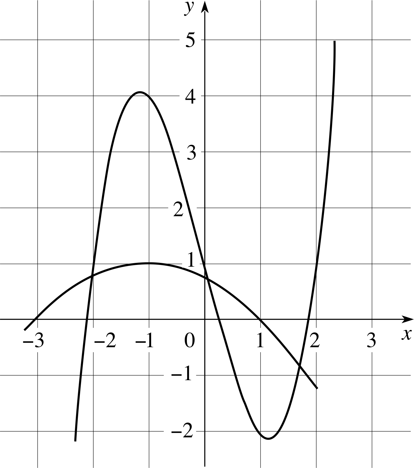
Figure 4 The graphs of Equations 26 and 27.
Since more function values must be calculated to plot the new graphs, it is probably better to go straight to one of the iterative methods discussed in the next subsection.
Any pair of simultaneous equations can be solved approximately by graphical methods. For example, the equations
y = x3 − 4x + 1(26)
and4y = 3 − 2x − x2(27)
can be solved by plotting the graphs of y = x3 − 4x + 1 and y = (3 − 2x − x2)/4. The points of intersection correspond to the solutions of this pair of equations. Figure 4 shows that there are three possible solutions, corresponding to the three intersections, at approximately
x = −2, y = 0.7
x = 0, y = 0.7
andx = 1.7, y = −0.8
which can be abbreviated to
(−2, 0.7), (0, 0.7), (1.7, −10.8) i
4.3 Numerical procedures
Figure 3 The graph of Equation 25.
Numerical procedures are methods of finding approximate solutions to a particular equation, in which all the constants are known numbers.
The bisection method
The simplest procedure, called the bisection method, is not much more than trial and error. If we want to solve the equation f (x) = 0, and we have some idea of the solution, perhaps from a graph, then we evaluate f (x) on either side of our initial estimate so as to obtain a range of x values over which the sign of f (x) changes. As an illustration, consider the equation
x3 − 4x + 1 = 0
corresponding to the function f (x) = x3 − 4x + 1.
From Figure 3 we see that there is a root between x = 1 and x = 2. This is confirmed by noticing that
f (1) = −2 and f (2) = 1
so that there is a sign change within the interval from x = 1 to x = 2.
At the mid–point, x = 1.5, we have f (1.5) = −1.625 so that the sign change (and therefore the root) must lie between x = 1.5 and x = 2.
Similarly, we can show that the root lies between x = 1.75 and x = 2; and we can continue in this fashion, bisecting the interval and evaluating the function at the mid–point, as far as we please and so obtain an approximation to the root which is as accurate as we need.
Regula falsi
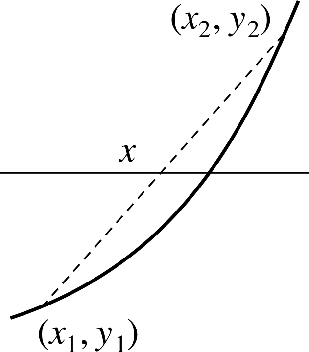
Figure 5 Regula falsi.
The method of bisection is very reliable and simple to implement as a computer program. It is true that it is comparatively slow, but with the speed of modern computers this hardly matters for a single calculation. However, speed may become a critical factor if you need to perform a large number of evaluations of roots. A simple method of speeding up the method considerably is the variation known as regula falsi. Let us look in detail at a graph of the neighbourhood of the solution, in Figure 5.
If x1 and x2 are initial estimates for the root, and if y1 = f (x1) and y2 = f (x2) have opposite signs, then a straight line between the two points will intersect the x–axis at a point which is closer to the root. The equation of the straight line joining the two points (x1, y1) and (x2, y2) is
$\dfrac{y-y_1}{x-x_1} = \dfrac{y-y_2}{x-x_2}$(28) i
If we put y = 0 in this equation, then the corresponding value of x will determine the point at which the line crosses the horizontal axis and will therefore give an improved estimate of the root. Thus,
$\dfrac{-y_1}{x-x_1} = \dfrac{-y_2}{x-x_2}$
which can be rearranged to give
$x=\dfrac{x_2 y_1 - x_1 y_2}{y_1-y_2}$
This improved estimate can be used as the starting point for an even better estimate.
Finding a root by this method takes fewer steps, although more work is required in each step. In practice it can be a fine judgement as to which method is more efficient in a particular case.
Question T19
The function defined in Equation 25 has a zero near x = 2.
f (x) = x3 − 4x + 1(Eqn 25)
Find this zero to an accuracy of five decimal places (i.e. so that the equation is satisfied to five decimal places) using one of the two numerical methods above. You may use your calculator.
Answer T19
The root is x = 1.860 81
Iterative methods
An alternative class of methods that are often useful are the iterative methods; these are based on the idea that if one has an approximate solution to an equation, then it can be used to get a better value. You might consider either of the previous methods to be in this class, but we usually mean methods in which the next approximation is obtained by a special formula. Look again at the equation x3 − 4x + 1 = 0, which we know, from Figure 3, has a solution near x = 2. We can rewrite the equation as
$x=\dfrac{2x^3-1}{3x^2-4}$(29) i
and we can use this to provide an iteration formula that relates an approximate root x n to a more accurate approximate root x n + 1
$x_{n+1} = \dfrac{2x^3_n-1}{3x^2_n-4}$(30)
So, if we set n = 1 in Equation 30 and take as our crude first approximation x1 = 2, we can use Equation 30 to find a better approximation x2 = 15/8 = 1.875. Setting n = 2 in Equation 30 we can now repeat this process (starting with x2 = 1.875) to find an even better approximation x3.
Continuing in this way we can obtain a succession of approximations x2, x3, x4, x5 and so on, with each step, or iteration, being an improvement on the last.
$\begin{align}x_2 &= 1.875\\x_3 &= 1.860\,978\,52\\x_4 &= 1.860\,805\,88\\x_5 &= 1.860\,805\,85\\x_6 &= 1.860\,805\,85\end{align}$ i
We stop when two successive iterations are the same to the required number of decimal places, since we can expect no further improvement.
Question T20
The equation $x^3+ 2x - 1 = 0$, which has a root near x = 0.45, can be rearranged to give
$x = \dfrac{1-x^3}{2}$
Using the first approximation x1 = 0.450 00 and the iteration formula
$x_{n+1} = \dfrac{1 - x_n^3}{2}$
find this root to five decimal place accuracy. (You may use your calculator.)
Answer T20
x1 = 0.450 00, x2 = 0.454 44, x3 = 0.453 08
x4 = 0.453 50, x5 = 0.453 37, x6 = 0.453 41
x7 = 0.453 39, x8 = 0.453 40, x9 = 0.453 40
Unfortunately, this simple method must be used with great care, and careful choice of the iteration formula is often needed to produce an iteration that will result in a meaningful answer. However, if the method does work, then it has the great advantage that it is almost proof against a mistake, since any reasonable approximation will be improved; the worst that can happen is that the process is slowed down somewhat.
More advanced methods, beyond the scope of this module, enable one to produce very rapid convergence to the root.
Question T21
The following iterative formula was used in the early days of computers to find the reciprocal of a given number a
xn+1 = xn(2 − axn)
Use this iteration to find 1/0.8 (i.e. let a = 0.8 in the above formula), starting with x1 = 1. (You may use your calculator.)
Answer T21
The sequence is 1, 1.2, 1.248, 1.249 9968, 1.250 000 00. It is characteristic of this method that the number of correct figures in the answer doubles at each stage.
5 Closing items
5.1 Module summary
- 1
-
Given a function f (x), a solution or root of the equation f (x) = 0 is a value of x that makes the equation true. Such a value is also a zero of the function and is represented graphically by any value of x at which the graph of f (x) meets the x–axis.
- 2
-
A Subsection 2.1linear equation in a single variable x has the general form ax + b = 0 and may be Subsection 2.1solved by rearrangement to give x = −b/a.
- 3
-
A pair of Subsection 2.3simultaneous linear equations may be solved by substitution; the method of elimination provides a standard routine for carrying out the substitution.
- 4
-
A set of simultaneous linear equations involving n unknowns may be solved, provided that it contains at least n independent equations and provided that none of the equations are inconsistent.
- 5
-
Simultaneous linear equations may also be solved Subsection 2.4graphically, by drawing appropriate straight lines and determining their point of intersection.
- 6
-
A quadratic equation ax2 + bx + c = 0 has roots $x = \dfrac{-b \pm \sqrt{b^2-4ac}}{2a}$, as may be demonstrated by the process of completing the square
- 7
-
If the discriminant, b2 − 4ac, of a quadratic equation is positive there are two real roots, if it is zero there is a repeated root, and if the discriminant is negative there are no real roots. In the latter case it is possible to find two Subsection 3.4complex roots of the form a + bi where $i = \sqrt{-1\os}$.
- 8
-
If the roots of ax2 + bx + c = 0 are α and β then α + β = −b/a and αβ = c/a. Such a quadratic may be factorized and written in the form (x − α)(x − β) = 0.
- 9
-
According to the fundamental theorem of algebra, a polynomial equation of degree n has n roots, provided we count complex roots and repeated roots.
- 10
-
Equations in general can be tackled by Subsection 4.2graphical, Subsection 4.3numerical and iterative techniques, but each case must be treated on its merits.
- 11
-
When solving equations that involve physical quantities, don’t introduce numbers until it is essential; leave all the arithmetic until the end.
- 12
-
Always check that your answers satisfy the original equations and that they make sense.
5.2 Achievements
After completing this module, you should be able to:
- A1
-
Define the terms that are emboldened and flagged in the margins of the module.
- A2
-
Solve simple linear equations by rearrangement.
- A3
-
Recognize an equation that is linear in a function of the unknown, and rearrange it for solution.
- A4
-
Solve linear simultaneous equations by substitution, provided they are consistent and independent.
- A5
-
Use graphical methods to solve simultaneous linear equations.
- A6
-
Recall the general form of a quadratic equation and sketch the graph of any given quadratic function.
- A7
-
Relate the coefficients of a given quadratic equation to the sum and product of the roots of that equation.
- A8
-
Factorize a simple quadratic function, and so solve the corresponding quadratic equation.
- A9
-
Explain the method of completing the square, and use it to solve a quadratic equation.
- A10
-
Write down the general formula for the roots of a quadratic equation, and use it to solve any particular equation.
- A11
-
Recall the definition of the discriminant, and explain how it determines the nature of the solutions of a quadratic equation.
- A12
-
Recall the nature and significance of complex numbers, and use them in the solution of quadratic equations.
- A13
-
Solve simple polynomial equations by factorization.
- A14
-
Describe the use of graphical methods in the solution of general equations, and use them to locate the roots of various equations.
- A15
-
Use the methods of bisection and regula falsi in the solution of simple equations. A16 Use iterative methods in the solution of equations given the iteration formula.
Study comment You may now wish to take the following Exit test for this module which tests these Achievements. If you prefer to study the module further before taking this test then return to the topModule contents to review some of the topics.
5.3 Exit test
Study comment Having completed this module, you should be able to answer the following questions, each of which tests one or more of the Achievements.
Question E1 (A2)
Find x if 2 (x − 1) + 3 (x − 6) = 0
Answer E1
x = 4
(Reread Subsection 2.1 if you had difficulty with this question.)
Question E2 (A3)
Find x if $\dfrac{1}{x-2}+2\left(\dfrac{1}{x-2}-6\right)=0$
Answer E2
If y = 1/(x − 2), then 3y = 12, y = 4. Then x − 2 = 1/4, and x = 9/4.
(Reread Subsection 2.2 if you had difficulty with this question.)
Question E3 (A4)
Solve the following simultaneous equations:
2x + y = −14, 3x + 5y = 1
Answer E3
x = −3, y = 2
(Reread Subsection 2.3 if you had difficulty with this question.)
Question E4 (A4 and A5)
Solve the following simultaneous equations first by drawing suitable graphs, then algebraically:
x + y = k, 2x − y = 1
for k = 2, 5 and 8.
Answer E4
Your graph(s) should show the straight line y = 2x − 1 and three lines y = k − x corresponding to values of k of 2, 5 and 8. The required solutions are the coordinates of the points of intersection.
(Of course, it is possible to work out the answers algebraically. To do so, it is sensible to first find the general solution in terms of k, namely x = (1 + k)/3 and y = (2k − 1)/3)
For the specified values of k:
if k = 2, then x = 1, y = 1
if k = 5, then x = 2, y = 3
if k = 8, then x = 3, y = 5
(Reread Subsection 2.4 if you had difficulty with this question.)
Question E5 (A6 and A11)
Sketch graphs to show quadratic functions with (a) two distinct zeros, (b) two coincident zeros, and (c) no real zeros.
Answer E5
These graphs are shown in Figure 2.
(Reread Subsection 3.1 if you had difficulty with this question.)
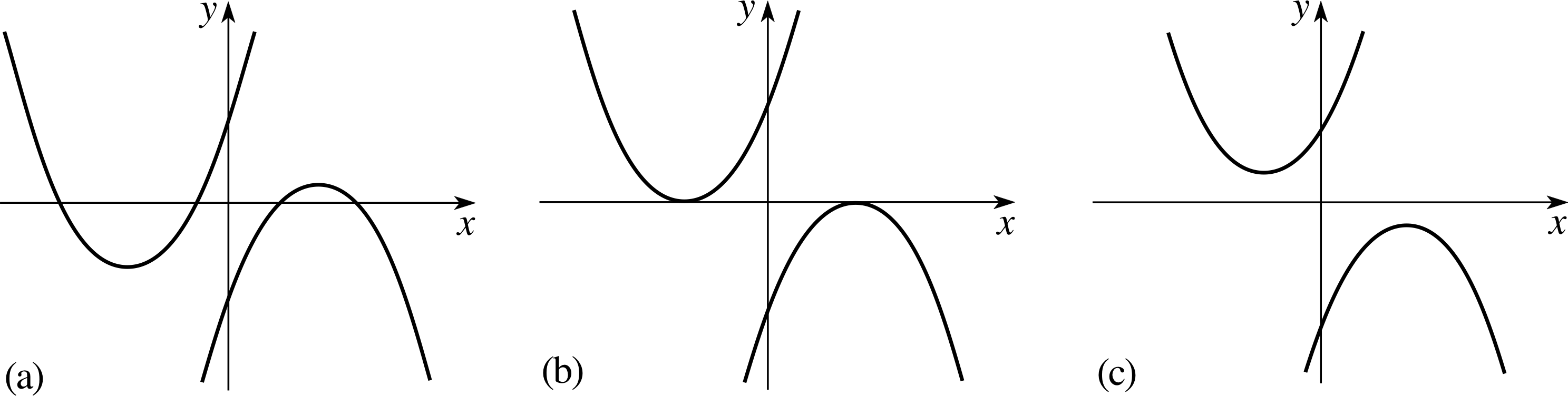
Figure 2 Graphs of six different quadratic functions.
Question E6 (A7 and A8)
Solve the following equations by factorizing the left–hand sides:
(a) x2 + 5x − 14 = 0 (b) 2x2 − 21x + 27 = 0
Check your answers by showing that the sum and product of the roots are correct in each case.
Answer E6
(a) (x − 2) (x + 7) = 0; so x = 2 or −7; sum of roots is −5, product of roots is −14.
(b) (2x − 3) (x − 9) = 0; so x = 3/2 or 9; sum of roots is 21/2, product of roots is 27/2.
Note that the sum and product of the roots are consistent with the coefficients of the equation in each case.
(Reread Subsection 3.2 if you had difficulty with this question.)
Question E7 (A9 and/or A10)
Solve the following equations:
(a) x2 − 2x − 1 = 0 (b) 3x2 + x − 2 = 0
Answer E7
(a) $x=1\pm\sqrt{2\os}$ (b) x = −1 or 2/3
(Reread Subsections 3.2 and 3.3 if you had difficulty with this question.)
Question E8 (A11)
State the conditions for the equation (in the variable x)
x2 − 2rx + s = 0
to have (a) two real roots, and (b) repeated roots.
Answer E8
The discriminant = 4 (r2 − s). If the discriminant is greater than zero, there are two real roots; if the discriminant is equal to zero there is a repeated root.
(Reread Subsection 3.3 if you had difficulty with this question.)
Question E9 (A10, A11 and A12)
Write down the roots of the equation in Question E8 above if neither of the conditions quoted there is fulfilled (so that the equation has complex roots).
Answer E9
In this case the discriminant is negative, and the roots may be written as $x=r\pm\sqrt{r^2-s}$ or $x = r\pm i \sqrt{s-r^2}$.
(Reread Subsection 3.4 if you had difficulty with this question.)
Question E10 (A13)
Guess one of the roots, and then solve the following equation by factorization:
x3 − 4x2 + x + 6 = 0
Answer E10
x = −1, +2, or +3
(Reread Subsection 4.1 if you had difficulty with this question.)
Question E11 (A14)
Sketch the graph of the function
g (x) = 3x3 − 11x2 + 5x + 8
and give approximate values for its zeros. (You may use your calculator.)
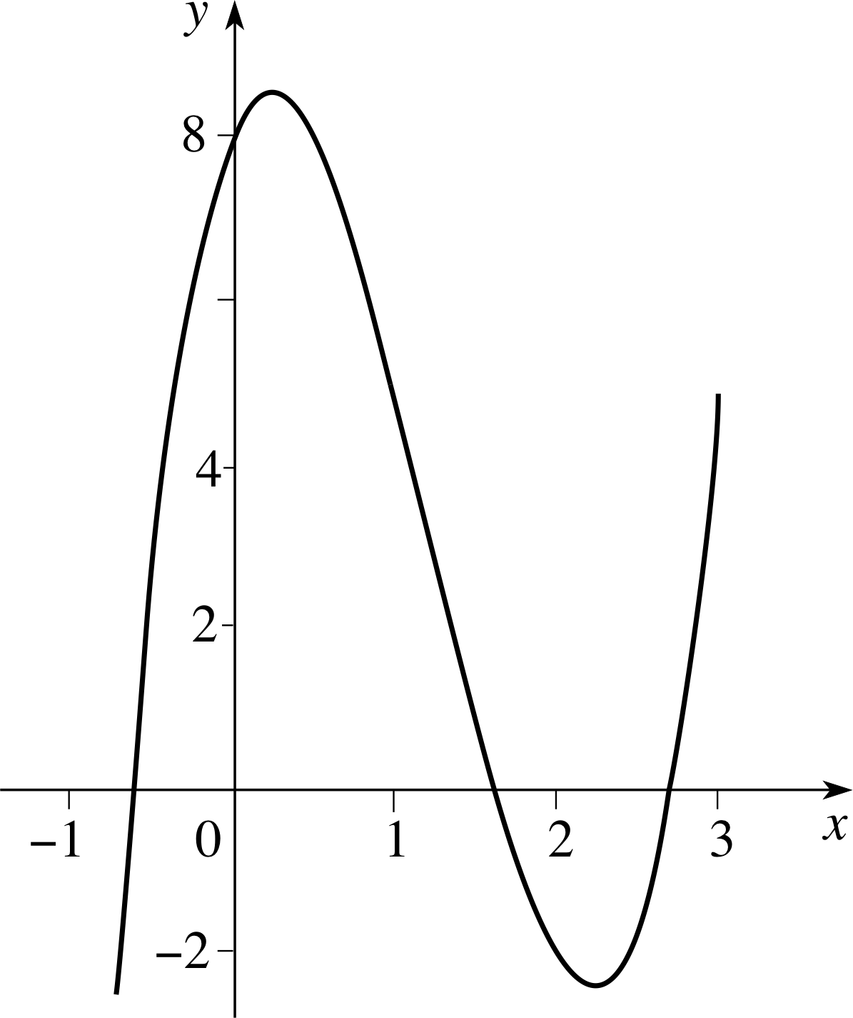
Figure 8 See Answer E11.
Answer E11
As Figure 8 indicates, the roots are approximately −0.6, 1.6, and 2.7
(Reread Subsection 4.2 if you had difficulty with this question.)
Question E12 (A15)
Use a numerical method (and the results of Question E11 above) to find the largest root of the equation
3x3 − 11x2 + 5x + 8 = 0
to two decimal places. (You may use your calculator.)
Answer E12
Using the method of bisection with starting values 2.65 and 2.75 quickly leads to a value of 2.67 to two decimal places. In fact the root is at x = 8/3.
(Reread Subsection 4.3 if you had difficulty with this question.)
Study comment This is the final Exit test question. When you have completed the Exit test go back and try the Subsection 1.2Fast track questions if you have not already done so.
If you have completed both the Fast track questions and the Exit test, then you have finished the module and may leave it here.
Study comment Having seen the Fast track questions you may feel that it would be wiser to follow the normal route through the module and to proceed directly to the following Ready to study? Subsection.
Alternatively, you may still be sufficiently comfortable with the material covered by the module to proceed directly to the Section 5Closing items.