MATH 4.1: Introducing differentiation |
PPLATO @ | |||||
PPLATO / FLAP (Flexible Learning Approach To Physics) |
||||||
|
1 Opening items
1.1 Module introduction
Many of the concepts and laws that physicists have to study involve the rate of change of one quantity with respect to another. Motion, which involves ideas such as position, velocity and acceleration provides many important examples. The velocity of an object is defined by the rate of change of its position with respect to time. The acceleration of an object is similarly defined by the rate of change of velocity with respect to time. In fact, rates of change are of such general importance that they have spawned an important branch of mathematics – differential calculus. This subject, created by Isaac Newton (1642–1727) and Gottfried Wilhelm Leibniz (1646–1716), allows the everyday notion of ‘rate of change’ to be made mathematically precise and has many applications throughout science and technology.
This module defines the important concept of the derivative and explains its role in evaluating rates of change. In Section 2 we adopt a graphical approach to rates of change and identify them with the gradients of tangents to graphs. This is done in the context of linear motion, introducing both velocity and acceleration as the gradients of appropriately constructed graphs. (The material in this section essentially repeats the discussion of linear motion in the physics strand of FLAP. If you have already studied that material you need only remind yourself of the terminology and the main results.)
Although the discussion in Section 2 is restricted to simple cases, this graphical approach is cumbersome and it is quite clear that a simple algebraic technique for evaluating gradients would be of great value. The mathematical process known as differentiation provides just such a technique, and it is here that the derivative enters the discussion. In Subsection 3.1 the link between functions and graphs (essentially the notion that a curve can be described by an equation) is used to introduce the idea of a derivative, while in Subsection 3.2Subsections 3.2 and Subsection 3.33.3 differentiation is introduced and used it to find some simple derivatives. A formal definition of the derivative is given in Subsection 3.4 and applied to velocity and acceleration in Subsection 3.5. Linear motion continues to provide the context and motivation throughout this discussion, but Subsection 3.6 goes on to show how derivatives can also be used in a wide variety of other circumstances.
Throughout this module the emphasis is on basic ideas and understanding rather than on complicated calculations. The main aim is that you should understand the mathematical approach to rates of change, be able to interpret derivatives such as $\dfrac{dx}{dt}$, $\dfrac{dv}{dt}$ and $\dfrac{dy}{dx}$ graphically, and evaluate them algebraically in straightforward situations. The full development of the techniques and applications of differentiation is left to other modules.
1.2 Fast track questions
Study comment Can you answer the following Fast track questions? If you answer the questions successfully you need only glance through the module before looking at the Subsection 5.1Module summary and the Subsection 5.2Achievements. If you are sure that you can meet each of these achievements, try the Subsection 5.3Exit test. If you have difficulty with only one or two of the questions you should follow the guidance given in the answers and read the relevant parts of the module. However, if you have difficulty with more than two of the Exit questions you are strongly advised to study the whole module.
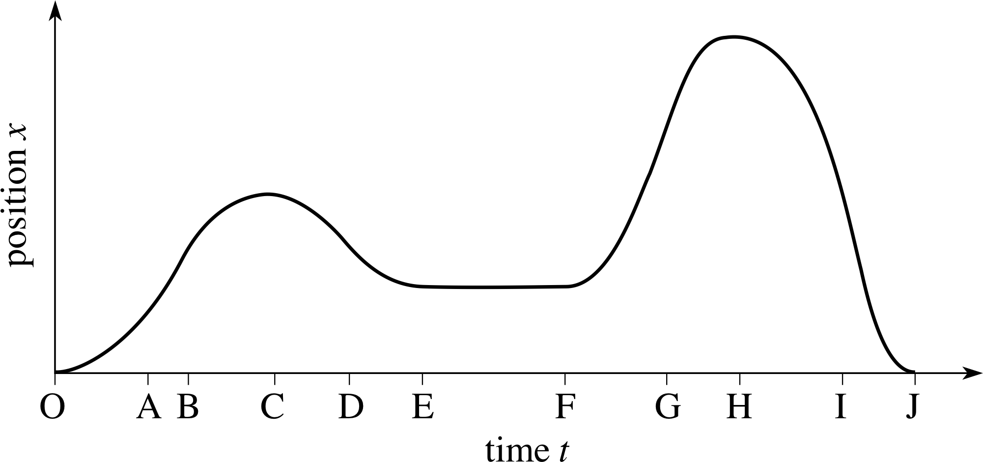
Figure 1 A graphical description of a car’s journey.
Question F1
Figure 1 is the position–time graph for a car moving along a straight road. Describe the car’s journey in everyday language.
During which parts of the journey is the acceleration (a) negative, (b) zero and (c) positive?
Answer F1
The car starts from rest at time 0 moving in the positive direction (forward), increasing its velocity until time A, at which point it travels at constant velocity until time B. Then it slows down, coming momentarily to a halt at C. It then reverses direction with increasing speed (the velocity is becoming more negative) until time D when it slows down, coming to a halt at time E. In remains stationary until time F when it moves forward, increasing its velocity until time G when it starts to slow and it momentarily stops and then reverses direction at time H. It now increases the speed with which it reverses (again, the velocity is becoming more negative) until I when it starts to slow and comes to a halt at its start point at time J.
(a) The acceleration is negative between B and D and between G and I.
(b) The acceleration is zero between A and B and between E and F.
(c) The acceleration is positive in the periods from O to A, D to E, F to G, I to J.
Question F2
The position x (t) of a body at time t is given by x (t) = −pt + qt2 where p and q are constants.
(a) Describe the nature and significance of dx/dt, write down its formal definition and use that definition to find an expression for dx/dt in terms of p, q and t.
(b) If p = 2 m s−1 and q = 3 m s−2, at what time is the velocity vx zero? What is the position at that time? What is the acceleration ax at that time?
Answer F2
(a) dx/dt is the rate of change of position with respect to time, i.e. the velocity v2. It is a function of time and at any particular time t its value is equal to the gradient of the tangent to the position–time graph at that time.
Its formal definition is
$\displaystyle \dfrac{dx}{dt} = \lim_{\Delta t \rightarrow 0}\left(\dfrac{\Delta x}{\Delta t}\right) = \lim_{\Delta t \rightarrow 0}\left[\dfrac{x(t+\Delta t)-x(t)}{\Delta t}\right]$
To apply this definition we calculate
x (t + ∆t) = −p (t + ∆t) + q (t + ∆t)2 = −pt − p (∆t) + qt2 + 2qt (∆t) + q (∆t)2
Sox (t + ∆t) − x (t) = − p (∆t) + 2qt (∆t) + q (∆t)2
Dividing both sides by ∆t gives
$\left[\dfrac{x(t+\Delta t)-x(t)}{\Delta t}\right] = -p + 2qt +q(\Delta t)$
So$\displaystyle \dfrac{dx}{dt} = \lim_{\Delta t \rightarrow 0}\left(\dfrac{\Delta x}{\Delta t}\right) = \lim_{\Delta t \rightarrow 0}\left[\dfrac{x(t+\Delta t)-x(t)}{\Delta t}\right] = -p + 2qt$
(b) The velocity is vx = −p + 2qt and is zero when $t = p/(2q) = \frac13$ s.
When $t = \rm \frac13\,s$
$x = \rm -2\,m\,s^{-1}\times\frac13\,s + 3\,m\,s^{-2}\times(\frac13\,s)^2 = -\frac13\,m$
The acceleration at this time is $a_x = \dfrac{dv_x}{dt} = 2q = \rm 6\,m\,s^{-1}$.
Study comment Having seen the Fast track questions you may feel that it would be wiser to follow the normal route through the module and to proceed directly to the following Ready to study? Subsection.
Alternatively, you may still be sufficiently comfortable with the material covered by the module to proceed directly to the Section 5Closing items.
1.3 Ready to study?
Study comment In order to study this module you will need to be familiar with the following terms: absolute value (or modulus), Cartesian coordinates, dependent variable, function, gradient, graph, independent variable, linear function and quadratic function. If you are uncertain of any of these terms you can review them by referring to the Glossary which will indicate where in FLAP they are developed. In addition, you will need to be familiar with SI units, and you must be able to determine the gradient of a straight–line graph. It is also assumed that you can carry out basic algebraic manipulations. The following questions will allow you to establish whether you need to review some of the topics before embarking on this module.
Question R1
On a set of two–dimensional cartesian_coordinate_systemCartesian coordinate axes plot the points A = (1, 1), B = (3, 3), C = (2, 6). Calculate the gradients of the lines AB, BC, AC.
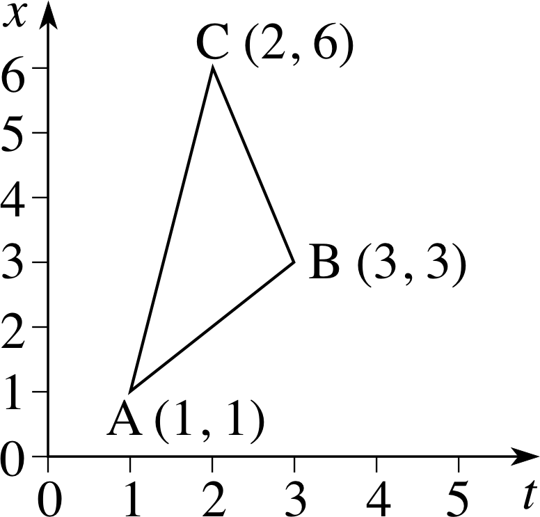
Figure 20 See Answer R1.
Answer R1
See Figure 20. The gradients of the lines are as follows:
$\text{gradient of AB} = \dfrac{\text{difference in }y\text{-coordinates}}{\text{difference in }x\text{-coordinates}} = \dfrac{3-1}{3-1} = 1$
$\text{gradient of BC} = \dfrac{\text{difference in }y\text{-coordinates}}{\text{difference in }x\text{-coordinates}} = \dfrac{6-3}{2-3} = \dfrac{3}{-1} = -3$
$\text{gradient of AC} = \dfrac{\text{difference in }y\text{-coordinates}}{\text{difference in }x\text{-coordinates}} = \dfrac{6-1}{2-1} = \dfrac51 = 5$
Comment If you are unsure of the answer to Question R1, consult graph and gradients in the Glossary.
Question R2
Draw the graph of the linear function x (t) = 1.2 + 3t. What is its gradient?
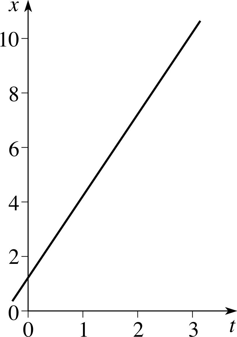
Figure 21 See Answer R2.
Answer R2
The graph of x (t) = 1.2 + 3t is given in Figure 21. The gradient is 3. This may be found from the coordinate differences between any two points on the line (as in Answer R1) or as the constant that multiplies t in the original function.
Comment If you are unsure of the answer to Question R2, consult graph and gradients in the Glossary.
Question R3
Draw the graph of the quadratic function x (t) = 5 + t + 3t2, for t ≥ 0.
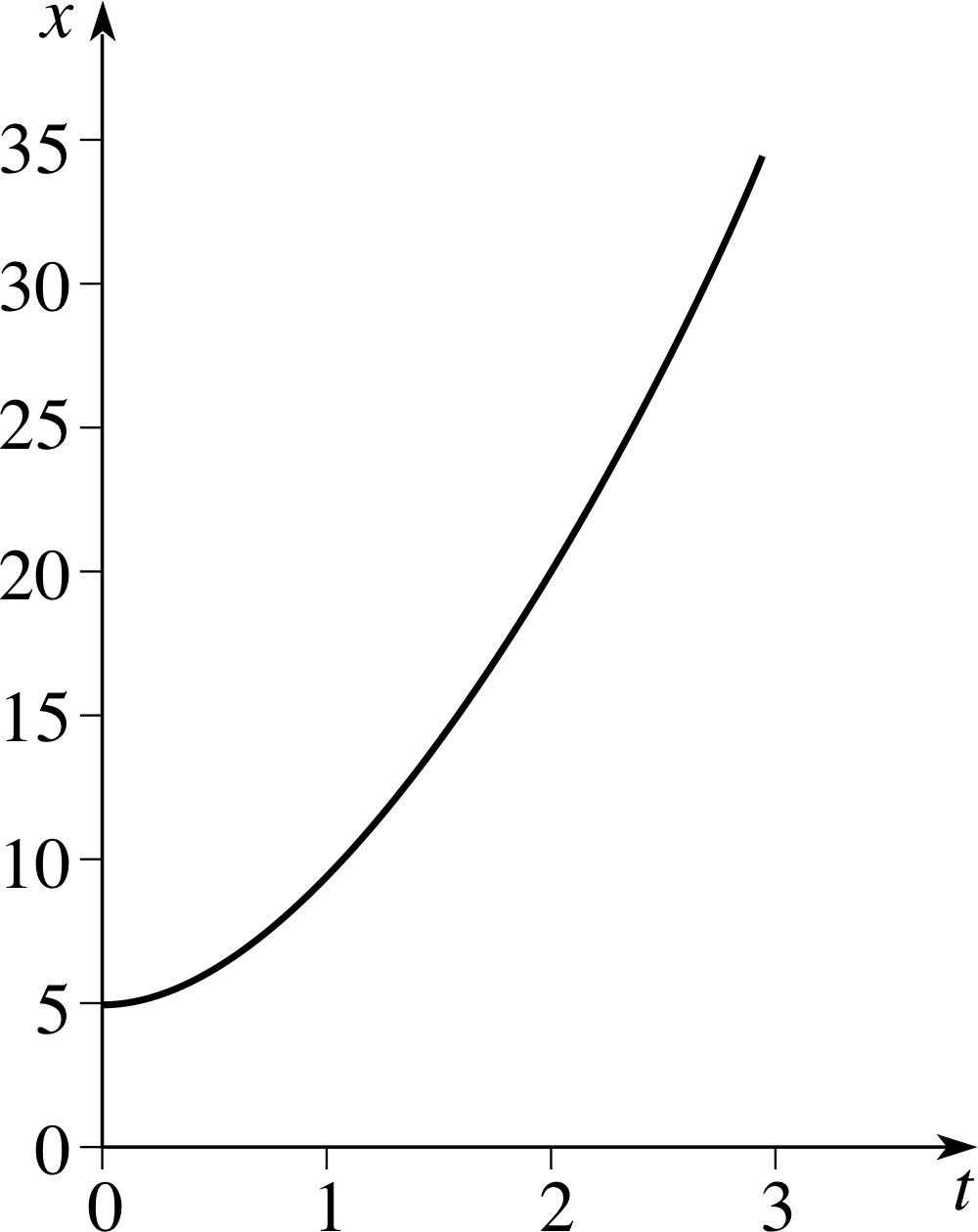
Figure 22 See Answer R2.
Answer R3
The graph of x (t) = 5 + t + 3t2 is given in Figure 22.
Comment If you are unsure of the answer to Question R3, consult graph and gradients in the Glossary.
Question R4
For the function x (t) = − 4 + 6t + 2t2, evaluate:
(a) x (0), (b) x (2), (c) | x (−1) |, (d) x (2.5) − x (2), (e) x (2.1) − x (2).
(f) If ∆t = 0.50, evaluate $\dfrac{x(2+\Delta t)-x(2)}{0.50}$
(g) If ∆t = 0.10 and t = 2, evaluate $\dfrac{x(t+\Delta t)-x(t)}{\Delta t}$
Answer R4
(a) x (0) = − 4 + 0 + 0 = −4
(b) x (2) = −4 + 6 × 2 + 2 × 4 = 16
(c) | x (−1) | = | −14 − 6 + 2 (−1)2 | = | −8 | = 8 (| x | should be read as ‘modulus of x’)
(d) x (2.5) − x (2) = −14 + 15 + 2 × 6.25 − 16 = 7.5
(e) x (2.1) − x (2) = −14 + 12.6 + 2 × 4.41 − 16 = 1.42
(f) $\dfrac{x(2+\Delta t)-x(2.0)}{0.50} =\dfrac{x(2.5)-x(2.0)}{0.50} = 7.50/0.50 = 15.00$
(g) $\dfrac{x(t+\Delta t)-x(t)}{\Delta t} =\dfrac{x(2.1)-x(2.0)}{0.10} = 1.42/0.10 = 14.20$
Comment Functions are reviewed briefly in this module, but if you are unsure about the answer to Question R4 you should consult function in the Glossary.
Question R5
Given that the variables x and t cover the same range of values, which (if any) of the following functions are equivalent?
(a) s (t) = 1 + 2t + t2, (b) y (x) = (1 + x)2, (c) v(t) = (1 − t)2 + 4t.
Answer R5
They all represent the same function. The letters are not important. Any other letters can be used provided they are always replaced consistently. So (b) can be written as s (t) = (1 + t)2 replacing y by s and x by t. But (1 + t)2 = 1 + 2t + t2 which is (a). Similarly, expanding and simplifying the right–hand side of (c) while replacing v by s also gives (a). (It is assumed that all the functions have the same codomain.)
Comment Functions are reviewed briefly in this module, but if you are unsure about the answer to Question R5 you should consult function in the Glossary.
2 Rates of change: graphs and gradients
Study comment The material in this section essentially repeats the discussion of linear motion given in the physics strand of FLAP. If you have already studied that material you need only remind yourself of the terminology and the main results before proceeding to Section 3 of this module.
2.1 Position–time graphs and constant velocity
Modern science is based on the idea that the world can only be understood by first making careful observations and measurements. Graphs provide an important way to represent such measurements. Although in the real world many things move along a curved path, it is obviously simpler to start with linear motion, i.e. motion along a straight line. This turns out to be less restrictive than it might initially appear, since any motion not involving spinning objects can be expressed as a combination of movements along two or three straight lines.
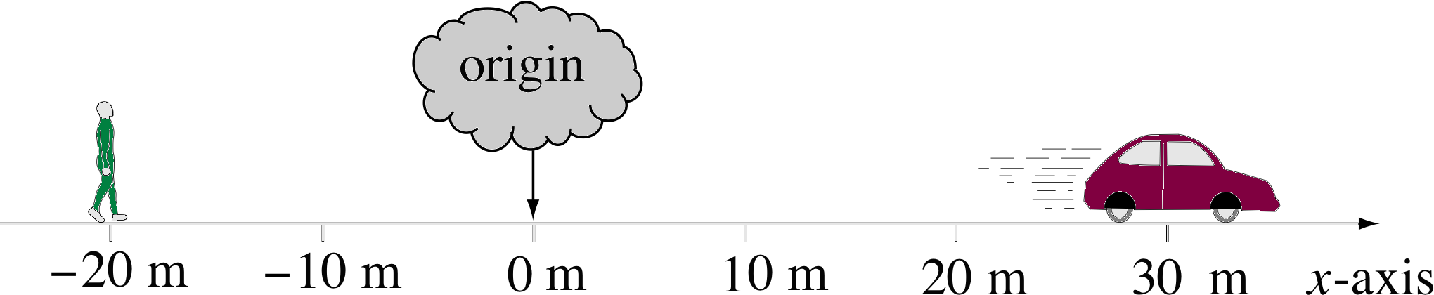
Figure 2 An example of one–dimensional motion.
| Position coordinate x/m |
Time t/s |
Position coordinate x/m |
Time t/s |
|---|---|---|---|
| 0 | 0.0 | 35 | 68.0 |
| 5 | 1.7 | 40 | 84.0 |
| 10 | 6.8 | 45 | 99.0 |
| 15 | 15.0 | 50 | 115.0 |
| 20 | 26.0 | 55 | 130.0 |
| 25 | 39.0 | 60 | 146.0 |
| 30 | 53.0 |
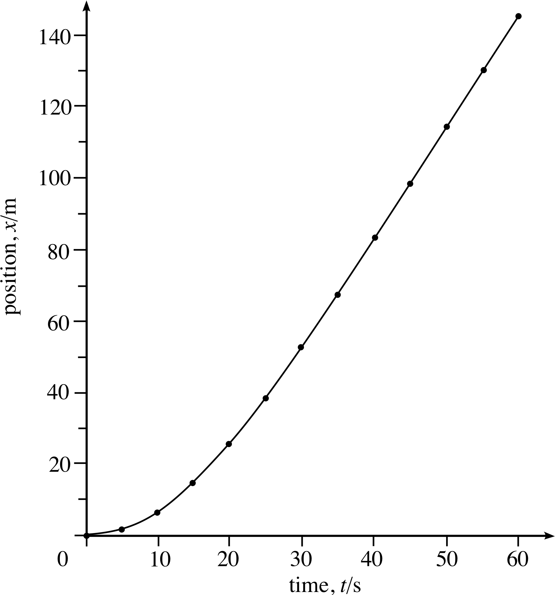
Figure 3 Position–time graph from Table 1.
Figure 2 shows a car and a pedestrian moving along a straight line. The line has been designated as the x–axis of some appropriately chosen system of Cartesian coordinates which has its origin at the fixed point indicated in the figure. At any time t, the position of the car or the pedestrian is completely specified by its position coordinate x which determines its displacement from the origin at that time. Note that x is measured in metres and may be positive or negative according to which side of the origin a point is located. At the particular instant pictured in Figure 2 the car is located at the point x = 30 m and the pedestrian is at x = −20 m. i
The position of a point automatically determines another quantity – its distance from the origin. This is the magnitude of its displacement from the origin. Of course, distances have to be positive quantities (it makes no sense to speak of a distance of −20 m) so we define the distance from the origin to any point on the line as | x |, the modulus or absolute value of its position coordinate. You will recall that absolute values are always positive, so | −20 m | = 20 m.
Table 1 shows the position of the car at 5-second intervals, starting from the time when it passed through the origin.
The corresponding graph, called the position–time graph of the motion, is shown in Figure 3. i As you can see, after about 30 s the graph is a straight line (i.e. linear) indicating that the car’s position coordinate is increasing by equal amounts in equal intervals of time. In other words, the rate of change of the car’s position with respect to time is constant after about 30 s.
Now, for an object moving along the x–axis, the rate of change of its position coordinate x with respect to time defines its velocity, vx, which tells us how fast it moves and in which direction. (If the object moves in such a way that x increases with time then vx is positive; if it moves in the opposite direction so that x decreases with time then vx is negative.) i So we can interpret the linear part of position–time graph as indicating that the car has a constant (or uniform) velocity after about 30 s.
✦ Using the data in Table 1 evaluate the car’s velocity vx in the time intervals from 40 s to 50 s and from 50 s to 60 s.
✧ From 40 s to 50 s, the position coordinate changes from 84 m to 115 m, so the velocity is
vx = (115 m − 84 m)/(50 s − 40 s) = 3.1 m s−1
From 50 s to 60 s, the velocity is
vx = (146 m − 115 m)/(60 s − 50 s) = 3.1 m s−1
Note that in this case the velocity is independent of the time interval over which it is evaluated, i.e. it is moving at a uniform velocity. Also note that the position coordinate is increasing with time so the velocity is positive.
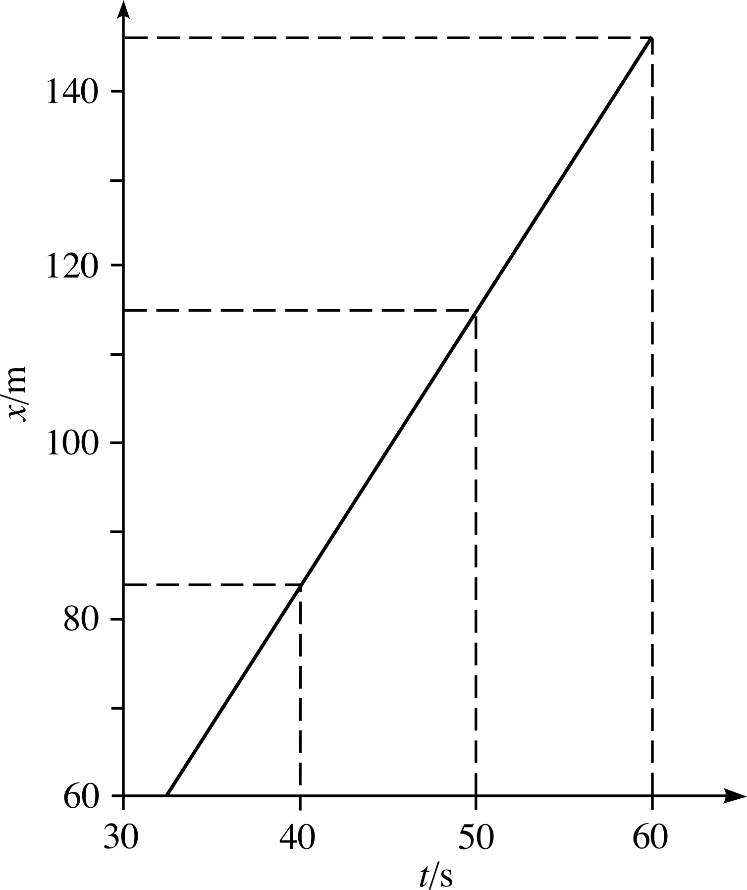
Figure 4 Enlarged segment of the linear portion of Figure 3.
✦ Figure 4 shows an enlargement of the linear part of Figure 3. How would you interpret the calculations performed in the last question in terms of Figure 4?
✧ Each of the calculations of velocity involved dividing the ‘rise’ of the graph (the change in x) by the corresponding ‘run’ (the corresponding change in t), i.e. finding the gradient of the straight line using the general formula
${\rm gradient} = \dfrac{\rm rise}{\rm run} = \dfrac{x_2-x_1}{t_2-t_1}$
We can summarize this discussion as follows:
For linear motion with uniform velocity, the position–time graph is linear, and the gradient of the position–time graph represents the rate of change of position with respect to time, i.e. the velocity.
Question T1
Construct a table similar to Table 1, and roughly sketch the corresponding position–time graph, when position coordinates are measured:
(a) from a new origin 20 m to the right of the old origin, with positions to the right defined as positive;
(b) from the new origin defined in part (a), but this time with positions to the left defined as positive.
How do your graphs relate to that of Figure 3?
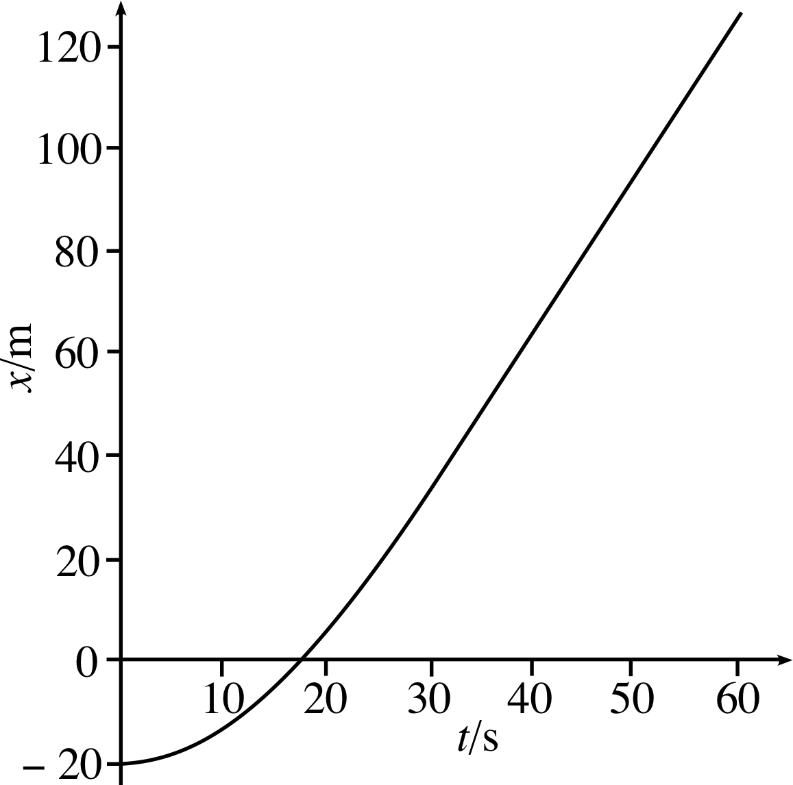
Figure 23 See Answer T1(a).
| Position coordinate x/m | Time t/s |
|---|---|
| 0 | -20.0 |
| 5 | −18.3 |
| 10 | −13.2 |
| 15 | −5.0 |
| 20 | 6.0 |
| 25 | 19.0 |
| 30 | 33.0 |
| 35 | 48.0 |
| 40 | 64.0 |
| 45 | 79.0 |
| 50 | 95.0 |
| 55 | 110.0 |
| 60 | 126.0 |
Answer T1
(a) The data are given in Table 6 and plotted in Figure 23. Figure 23 is Figure 3 shifted downwards. Different choices of reference point (the origin) simply shift the position–time graph upwards or downwards without changing its shape. The new choice of origin has not affected the gradient, so the velocities found using this graph would be exactly the same as those from Figure 3.
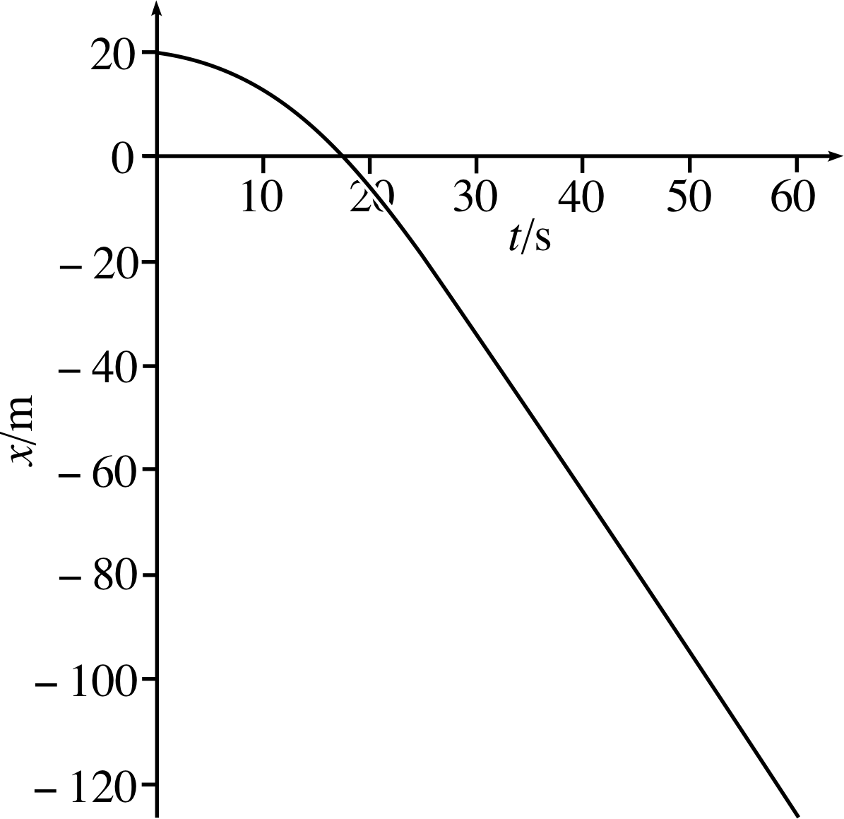
Figure 24 See Answer T1(b).
| Position coordinate x/m | Time t/s |
|---|---|
| 0 | 20.0 |
| 5 | 18.3 |
| 10 | 13.2 |
| 15 | 5.0 |
| 20 | −6.0 |
| 25 | −19.0 |
| 30 | −33.0 |
| 35 | −48.0 |
| 40 | −64.0 |
| 45 | −79.0 |
| 50 | −95.0 |
| 55 | −110.0 |
| 60 | −126.0 |
(b) The data are given in Table 7 and plotted in Figure 24. Figure 24 is Figure 23 turned upside down. Reversing the choice of positive direction turns the graph upside down. The choice of positive direction affects the sign of the gradient and hence velocities found from this graph will have the opposite sign to those found using Figure 23 – the car is now travelling in the negative direction so its velocity is negative.
An important point to notice about motion along the x–axis with uniform velocity vx is that it implies that the moving object is always travelling in the same direction. Sometimes we may want to know how rapidly an object is moving but we may not care about its direction of motion. Under such circumstances the quantity likely to interest us is the speed of the object, given by
v = | vx | = magnitude of velocity
Since | vx | can never be negative it is clear that the speed v can never tell us anything about the direction of motion. Objects moving in opposite directions with velocities of 20 m s−1 and −20 m s−1 will both have a speed of 20 m s−1.
Question T2
Figure 5 shows the position–time graphs for four different bodies each moving with a different constant velocity along the x–axis. If you assume the position and time scales are the same in each case:
(a) Arrange the bodies in order of increasing speed.
(b) Which body has the greatest velocity?
(c) Which body has the least velocity?
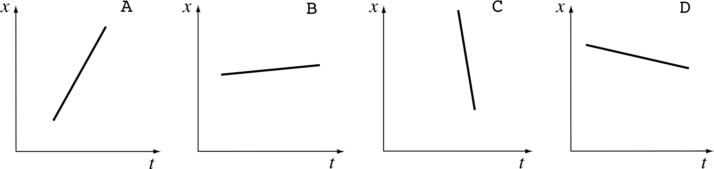
Figure 5 See Question T2.
Answer T2
(a) The steeper the graph, the greater the change in position in a given interval of time, and therefore the greater the speed. So in terms of increasing speed the order is B, D, A, C.
(b) Graphs A and B have positive gradients (since x increases as t decreases). The gradient of A is greater (i.e. more positive) than B, therefore A has the greatest velocity of the four.
(c) Graphs C and D have negative gradients (since x decreases as t increases). The gradient of C is more negative than D, therefore C has the least velocity of the four.
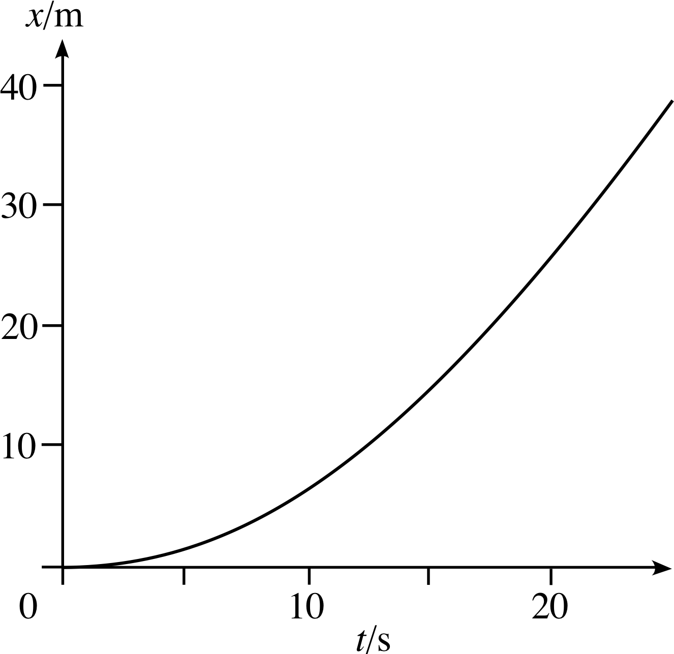
Figure 6 Enlargement of the curved portion of Figure 3.
2.2 Position–time graphs and instantaneous velocity
You saw in the last subsection that the gradient of a linear position– time graph can represent a constant velocity. This idea of using gradients is also the key to dealing with velocities that are not constant. Figure 6 is an enlargement of Figure 3 in the interval from 0 to 20 s. In this case the graph is curved which indicates that the velocity is changing. As you will see it is still true that the velocity at any particular time is given by the gradient of the graph at that time, but what exactly do we mean by the gradient at a particular time when the graph is curved? For example, in Figure 6, what is the gradient of the curve at t = 5 s? The definition of the gradient at a point on a curved graph occupied Newton and Leibniz, the founders of the calculus, more than a little and we will now consider that question in the context of position–time graphs.
How should we set about finding the velocity of the car at t = 5 s? Let’s try something similar to our approach in the last subsection.
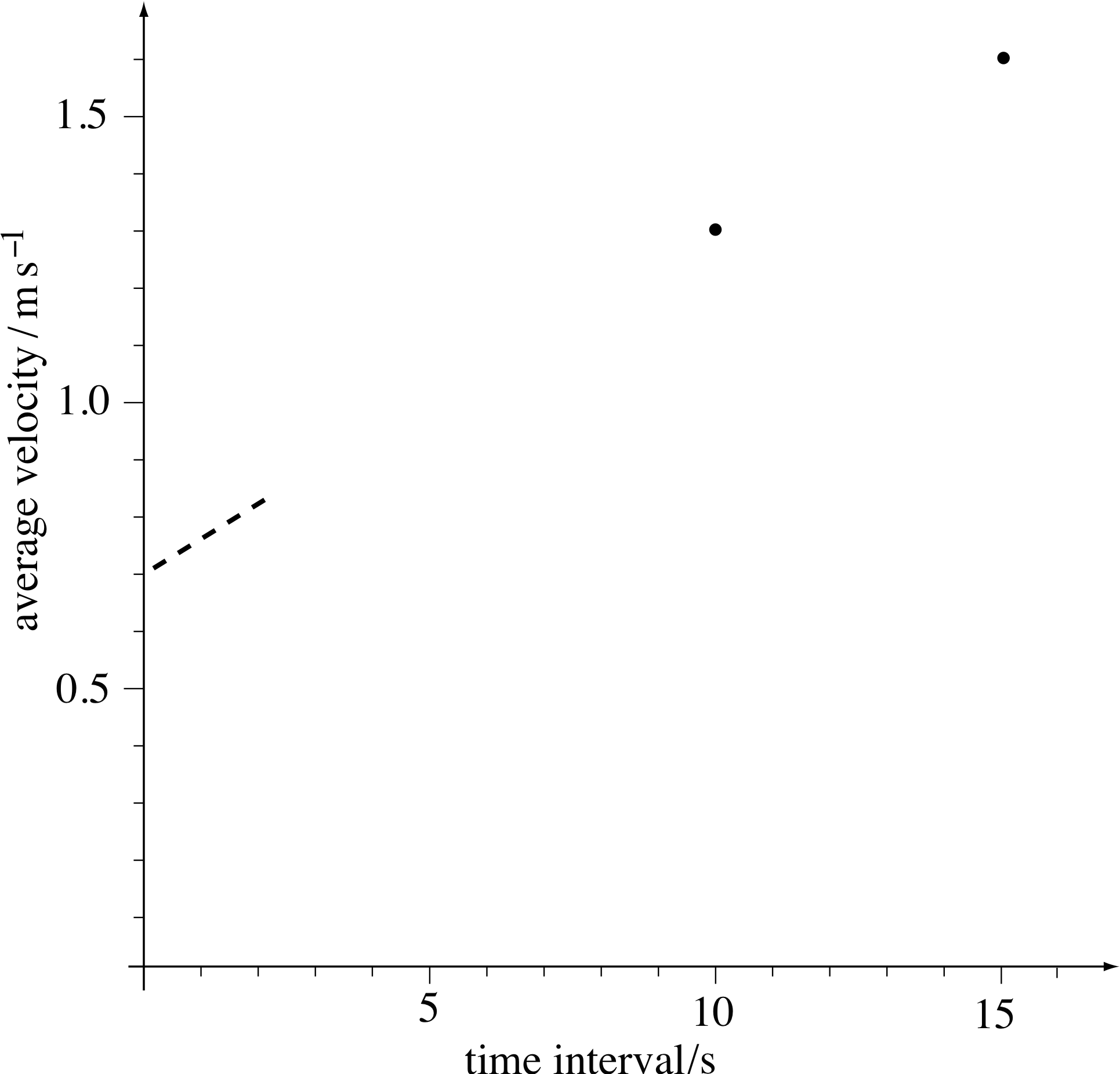
Figure 7 The average velocities of the car plotted against the duration of the time intervals over which they have been computed.
In the 15 s interval from 5 s to 20 s the position coordinate changes by 24.3 m, from 1.7 m to 26.0 m. If we divide the change in position coordinate by the time interval we get the average velocity $\langle v_x\rangle$ over that time interval.
So, over the interval from 5 s to 20 s,
$\langle v_x\rangle$ = 24.3 m/15 s = 1.6 m s−1
We can now measure the average velocity over a shorter interval starting at 5 s. For example, over the interval from 5 s to 15 s, the change in position coordinate is 13.3 m.
So, over the interval from 5 s to 15 s,
$\langle v_x\rangle$ = 13.3 m/10 s = 1.3 m s−1
The values are plotted in Figure 7
In principle we could go on like this, using shorter and shorter intervals, but in practice it becomes impossible to continue when the interval becomes so short that the change in position coordinate cannot be reliably determined from the graph. Fortunately, we do not really need to do that as you are about to see.
Question T3
Using Figure 6, determine as accurately as you can the average velocities over the following intervals: (a) 5 s to 10 s, (b) 5 s to 9 s, (c) 5 s to 8 s. Then plot the three additional points on the graph in Figure 7.
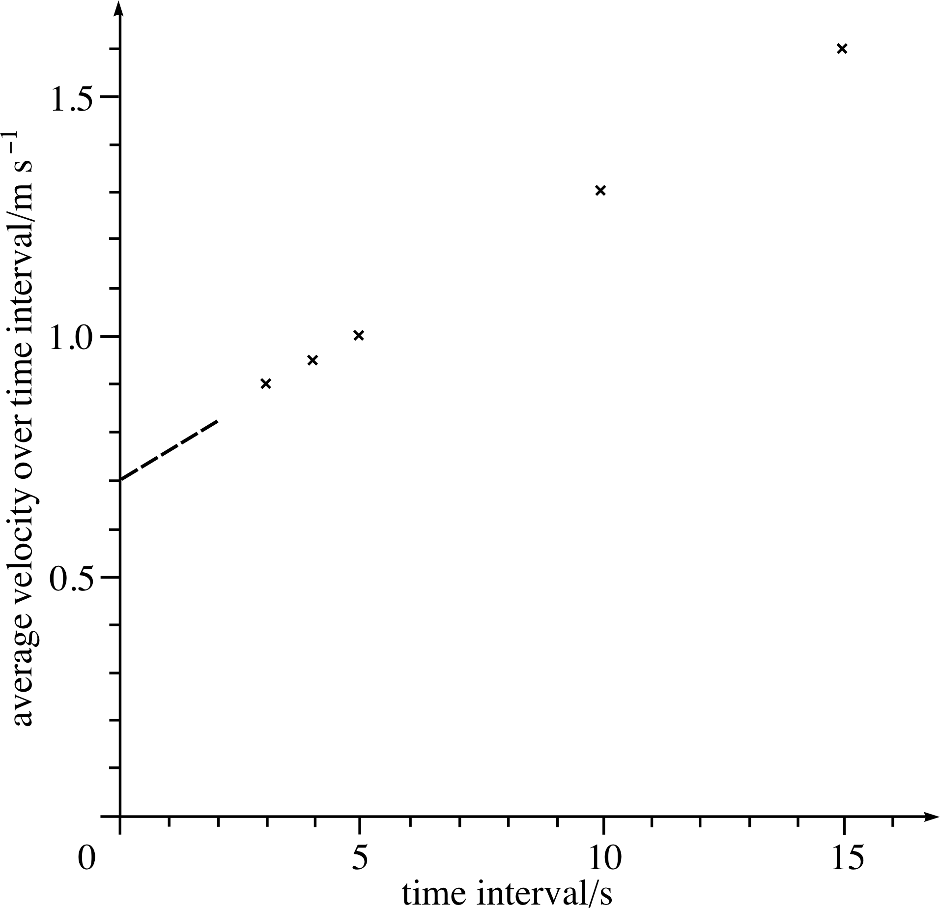
Figure 25 See Answer T3.
Answer T3
You should obtain the values given in Table 8, to within an uncertainty of about 5%, or so. Figure 25 shows the points from Table 8 added to Figure 7.
| Interval | Average velocity |
|---|---|
| 5.0 s to 10.0 s | (7.0 m − 1.8 m)/(10.0 s − 5.0 s) = 1.0 m s−1 |
| 5.0 s to 9.0 s | (5.5 m − 1.8 m)/(9.0 s − 5.0 s) = 0.95 m s−1 |
| 5.0 s to 8.0 s | (4.5 m − 1.8 m)/(8.0 s − 5.0 s) = 0.90 m s−1 |
Now imagine using intervals starting at 5 s that are much shorter than those in Question T3 to evaluate some more average velocities.
✦ Where do you think these points would lie on the graph of Figure 7?
✧ They would lie on the dashed line shown, which cuts the axis at about 0.70 m s−1.
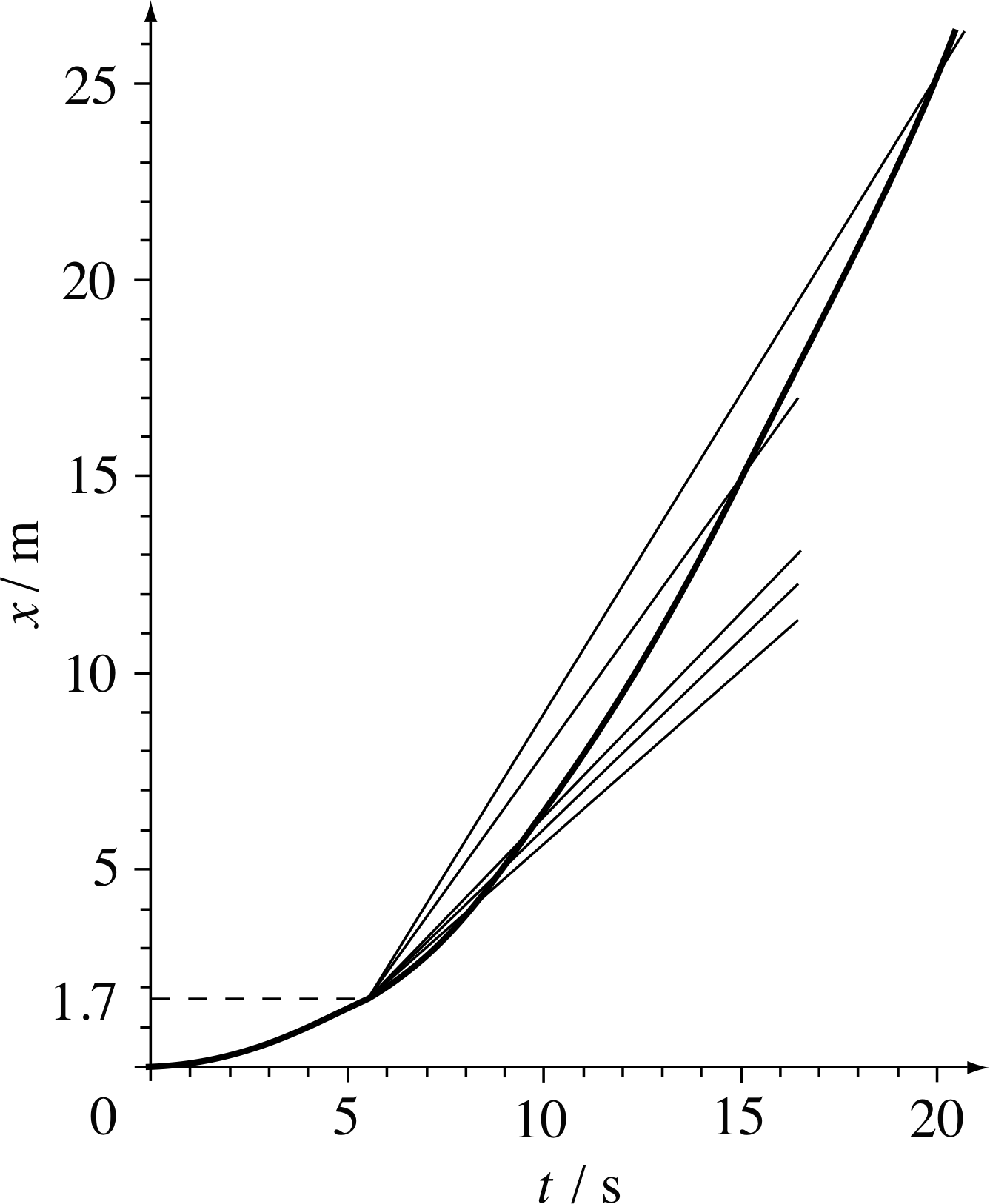
Figure 8 The average velocities plotted on Figure 7 are the gradients of the lines passing through the point corresponding to time t = 5 s.
The velocity of 0.70 m s−1 is called the limit of the average velocity, i.e. the value that is reached as the time interval from 5 s is made smaller and smaller. This limit gives us a definition of the instantaneous velocity at any particular moment:
instantaneous velocity at time t = the limit of the average velocity over an interval around t as that interval is made smaller and smaller
Note that by means of this limiting procedure we are able to make sense of the phrase ‘instantaneous velocity’ even though the moving object can’t really travel any distance at all in an ‘instant’. In general, ‘the velocity’ of an object is taken to refer to its instantaneous velocity at a particular time. Likewise, ‘the speed’ is generally taken to refer to the instantaneous speed, i.e. the magnitude of the (instantaneous) velocity.
It is useful to view what we have done in terms of the gradients of chords, i.e. straight lines that cut the curve at two points.
In Figure 8, the upper straight line passes through the points on the graph corresponding to the times t = 5 s and t = 20 s. The gradient of this straight line is the average velocity over that time interval. Other average velocities over shorter intervals are given by the gradients of the other lines in Figure 8, each of which cuts the curve at the beginning and endpoint of the relevant interval. As the intervals become smaller and smaller the lines crowd together and become nearly indistinguishable from one another. This corresponds to the average velocity becoming closer and closer to its limit.
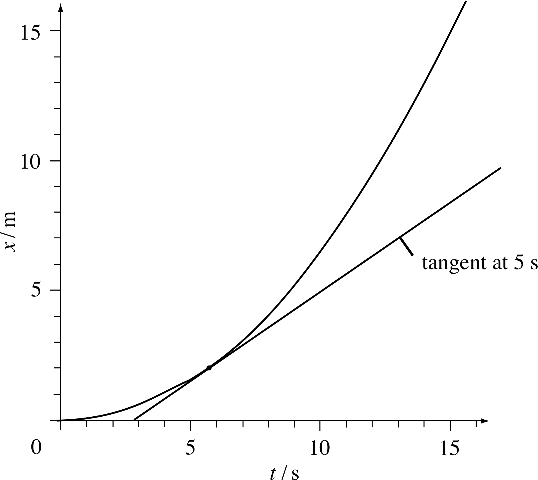
Figure 9 The instantaneous velocity of the car at t = 5 s is the gradient of the tangent to the graph at t = 5 s.
Figure 9 shows the straight line that just touches the graph at 5 s. This line is the ‘limit’ of the lines drawn in Figure 8. It is called the tangent_to_a_curvetangent at t = 5 s, and its gradient gives the instantaneous velocity at t = 5 s.
✦ Measure the gradient of the tangent at 5 s in Figure 9.
✧ The answer is approximately 0.70 m s−1, the instantaneous velocity deduced from Figure 7.
Although limited in accuracy because of the difficulty of drawing tangents we now have an alternative definition of the instantaneous velocity. At any time t:
instantaneous velocity = gradient of the tangent to the position–time graph
Eventually, this approach will allow us to develop an algebraic technique which is much easier to apply than the graphical method, but before doing that we will consider how the ideas we have already developed allow us to deal with acceleration.
2.3 Velocity–time graphs and instantaneous acceleration
Table 2 shows the measured velocity vx at six instants for a ball falling freely from rest. Just as Table 1 was used to plot a position–time graph, so we can use Table 2 to obtain the velocity–time graph shown in Figure 10.
In this case, the graph is a straight line, i.e. for any given interval of time the velocity changes by a constant amount. The rate of change of velocity with respect to time is called acceleration, and it can be found from the gradient of the velocity–time graph. i Figure 10 shows that for our freely–falling ball the acceleration in the first second is constant or uniform.
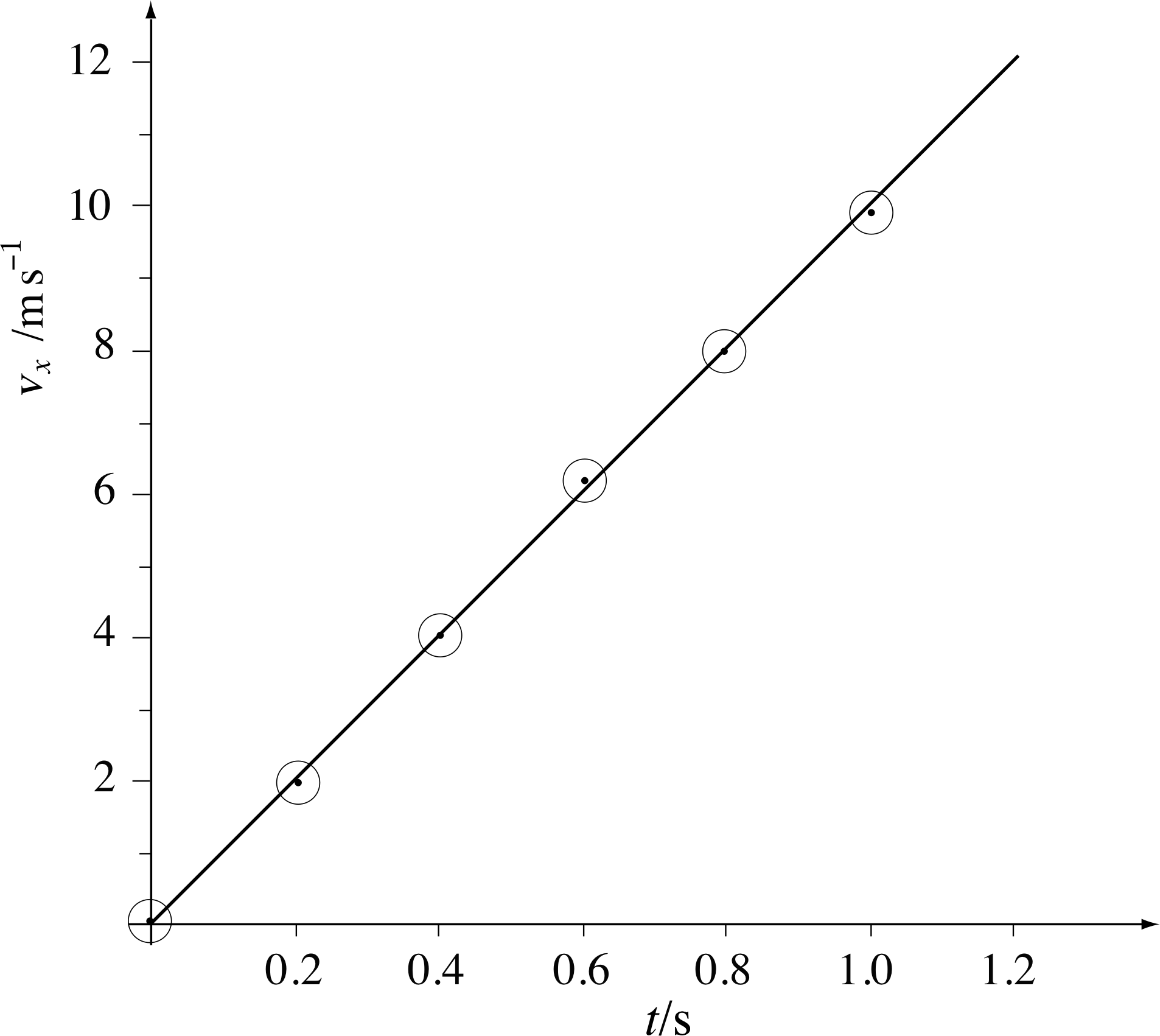
Figure 10 The velocity–time graph of a falling ball for the first second after release.
For linear motion with constant (or uniform) acceleration, the velocity–time graph is linear, and its gradient represents the rate of change of velocity with respect to time, i.e. the acceleration.
| Time from release t/s |
Velocity of falling ball vx1/ m s−1 |
|---|---|
| 0.0 | 0.00 |
| 0.2 | 1.97 |
| 0.4 | 3.93 |
| 0.6 | 6.10 |
| 0.8 | 7.81 |
| 1.0 | 9.80 |
✦ What is the gradient of the linear graph in Figure 10? (Take care to include the appropriate SI units.)
✧ The gradient is approximately 10 m s−2.
(The units are (m s−1)/s = m s−2).
Acceleration, like velocity, has direction as well as magnitude. By giving the velocities in Table 2 a positive sign, we are saying that the downwards direction is positive and, since the velocities are increasing with time, the acceleration is also positive. If the velocities were decreasing in magnitude, but still positive, the acceleration would be negative.
It’s worth noting that a negative acceleration does not always slow things down, as the following question shows.
✦ Suppose an object is moving in the negative x–direction and it is subject to a negative acceleration. Does the magnitude of its velocity (i.e. its speed) increase or decrease?
✧ The initial velocity is negative and negative acceleration will make this more negative – but the magnitude of the velocity (i.e. speed) will increase.
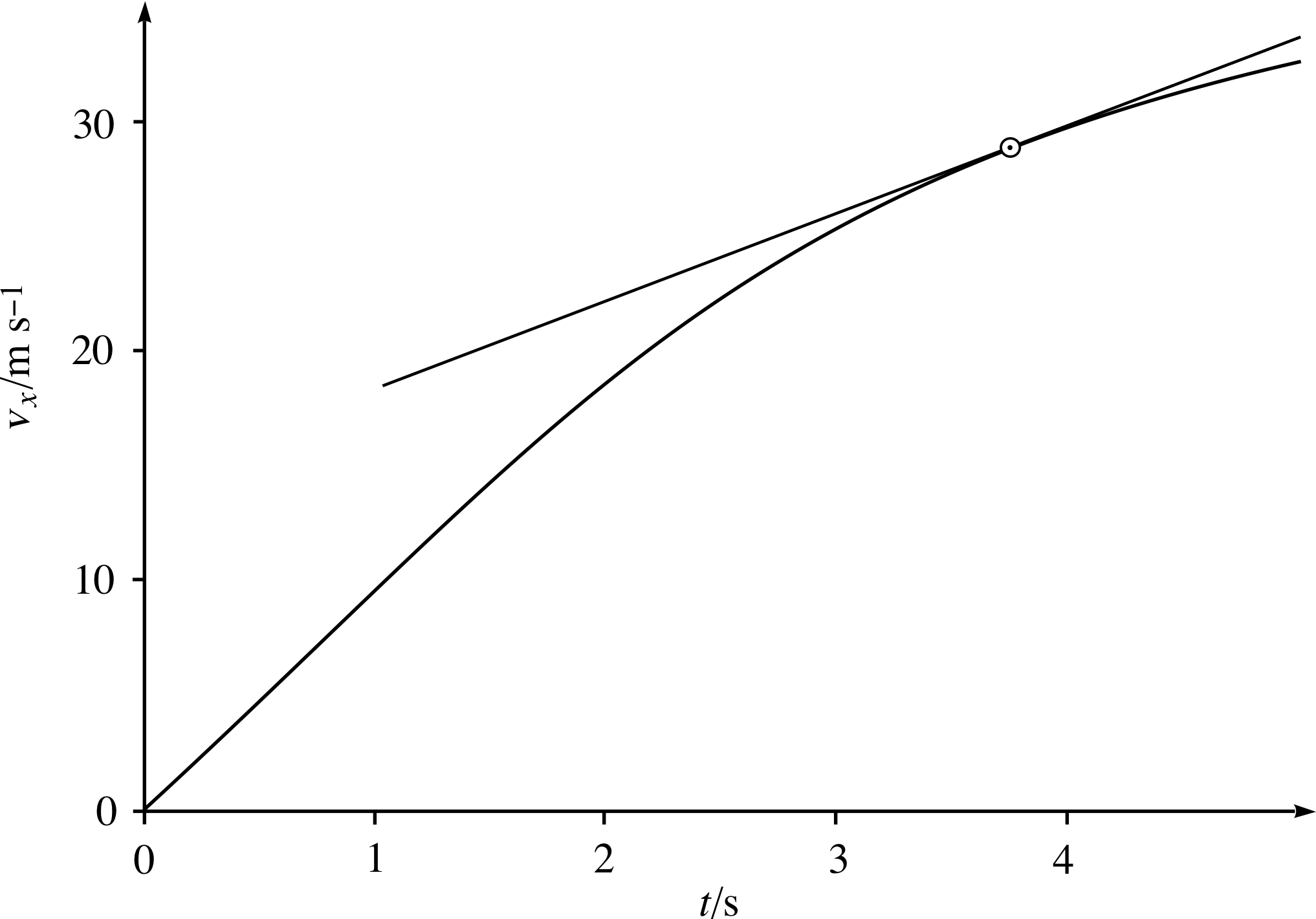
Figure 11 The velocity–time graph of a falling ball. The gradient of the tangent line at 3.75 s gives the instantaneous acceleration of the ball at 3.75 s.
The term deceleration is often used to describe the slowing down of a body. It is sometimes stated that deceleration is negative acceleration but, as the question above shows, that is not necessarily the case – a negative acceleration only causes a reduction in speed if the motion is in the direction defined as positive.
Accurate measurement of the acceleration of freely–falling objects in the absence of air resistance gives a value of 9.8 m s−2 (to two significant figures). However, our ball is not falling in a vacuum so air resistance i tends to slow its fall, as Figure 11 shows. After a few seconds the graph curves, rising less and less steeply. Hence the velocity is increasing less rapidly and the acceleration is no longer constant. (This is because the air resistance becomes greater as the ball’s velocity increases.)
Faced with this changing acceleration we can take the same approach to instantaneous acceleration as we took to instantaneous velocity: draw a tangent to the curve at the relevant time and measure its gradient. In Figure 11 a tangent has been drawn at the point on the curve where the time is 3.75 s. The tangent has a gradient of 3.9 m s−2, so this is the instantaneous acceleration of the ball at 3.75 s. So, for linear motion, at any time t:
instantaneous acceleration = gradient of the tangent to the velocity–time graph
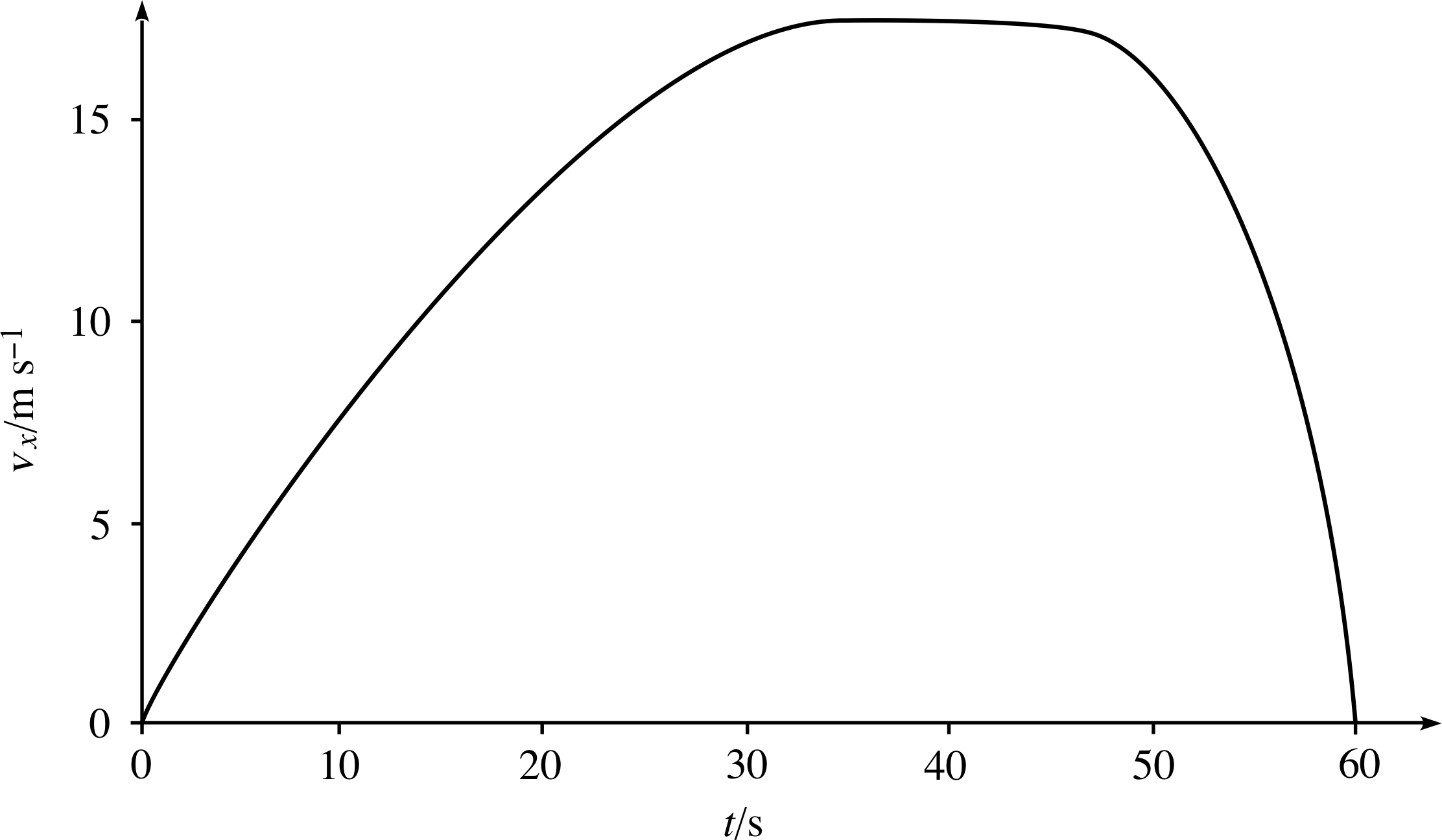
Figure 12 See Question T4.
Question T4
Figure 12 shows the velocity–time graph of a car on a short journey along a straight road. Measure the instantaneous acceleration at 10 s, 40 s and 55 s. Give a one–sentence description of the journey using everyday language.
Answer T4
By drawing tangents at 10 s, 40 s and 55 s and measuring their gradients the accelerations are found to be 0.66 m s−2, 0 m s−2 and −1.3 m s−2, respectively.
The car accelerates from rest to a steady velocity of 17.5 m s−1 in about 34 s, remains at that velocity for about 10 s, and then decelerates to rest in about a further 15 s.
2.4 Gradients and rates of change in general
The crucial relationship in our discussion has been between the gradient of a tangent at a point on a curve and a rate of change. The gradient of the tangent at a point on the position–time curve gives the rate of change of position with respect to time, i.e. the instantaneous velocity, at the time corresponding to where the tangent is drawn. The gradient of the tangent at a point on the velocity–time curve gives the rate of change of velocity with respect to time, i.e. the instantaneous acceleration, again at the time corresponding to where the tangent is drawn. This approach works in many other situations. For example, if we have a graph showing how the temperature of an object changes with time then the gradient of the tangent at a point on that graph gives the instantaneous rate of change of temperature with respect to time at that specific time. The gradients of the tangents at different points on the curve give the rates of change of temperature at different times. Although the expression ‘rate of change’ is used, the quantity plotted horizontally need not be time. If temperature is plotted against altitude then drawing a tangent to the curve and finding its gradient will give the rate of change of temperature with respect to altitude at the altitude corresponding to the point where the tangent is drawn. Another example is the plot of the magnitude of the force exerted by a spring against its extension. Again the gradient at any point gives the rate of change of force magnitude with respect to extension at that point.
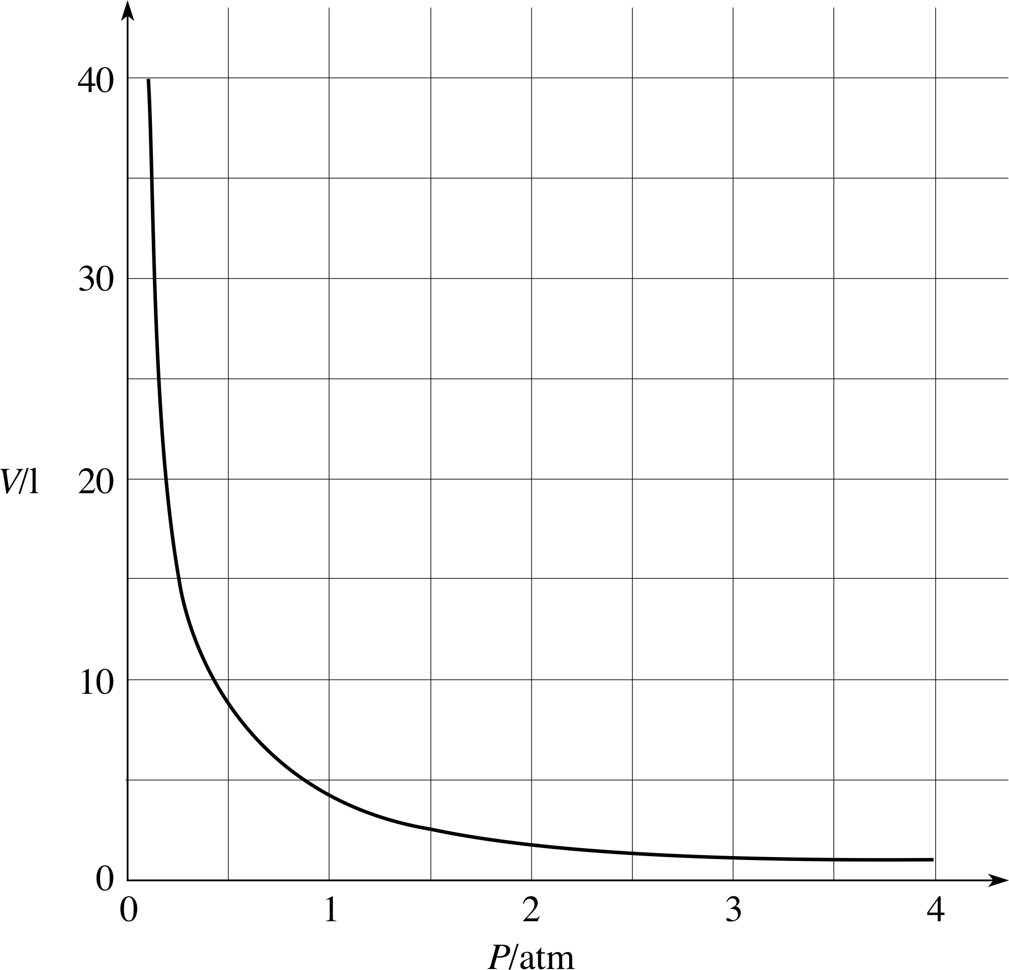
Figure 13 See Question T5.
Question T5
Figure 13 shows a graph of the volume V of a sample of gas against its pressure P (V is measured in litres (l) and P in atmospheres (atm)). i Estimate the rate of change of volume with respect to pressure at P = 1 atm. What happens to the rate of change of volume with respect to pressure as the pressure increases? What happens to the rate of change of pressure with respect to volume as the volume increases?
Answer T5
The rate of change of volume with respect to pressure is approximately −4.5 litres atm−1 and is given by the gradient of the tangent to the curve at P = 1 atm. As the pressure increases the rate of change of volume with respect to pressure increases (i.e. becomes less negative). To find the rate of change of pressure with respect to volume you really need a graph of P against V, though you might be able to imagine what it looks like from Figure 13. In any event, the rate of change of pressure with respect to volume is also negative and it too increases (i.e. becomes less negative) as the volume increases since the gas becomes easier to compress and a given increase in volume corresponds to a smaller and smaller reduction in pressure.
3 Rates of change: functions and derivatives
Section 2 should have convinced you that determining the gradients of tangents can provide useful information in many situations. However, performing this task graphically is very tedious and not always precise. Fortunately there is a non–graphical technique for calculating gradients that can be applied if we know the equation that describes the shape of a graph. This technique is called differentiation. It is part of that branch of mathematics known as calculus and was developed initially to study motion. In this section, we will briefly review the concept of a function and then introduce differentiation.
3.1 Functions, graphs and derivatives
Crudely speaking, a function is a rule (usually written as an algebraic equation) that relates two sets (usually sets of numbers or values). For example, the rule x = t2 relates any real number t to a non–negative real number x. We show that x is determined by t by writing
x (t) = t2 for any real number t
and we say that x is a function of t. For any value of t we can use the given rule to work out a corresponding value of x; if t = 2 then x = 4, if t = 3 then x = 9 and so on. (Note that when we write x (t) in this context we do not mean x × t.)
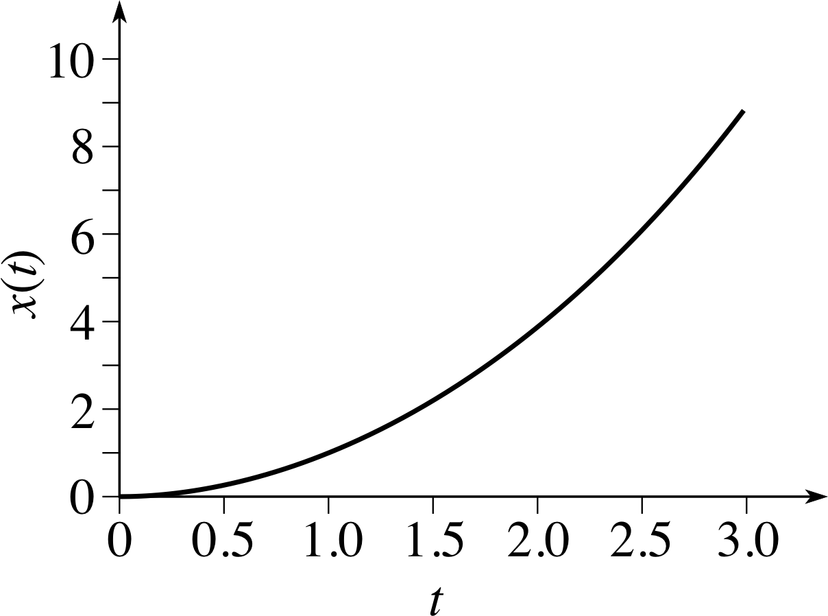
Figure 14 The graph of the function x (t) = t2.
| t | x (t) |
|---|---|
| 0.0 | 0.00 |
| 0.5 | 0.25 |
| 1.0 | 1.00 |
| 1.5 | 2.25 |
| 2.0 | 4.00 |
| 2.5 | 6.25 |
| 3.0 | 9.00 |
When dealing with functions of this kind we call x and t variables and we say that x is a dependent variable, the value of which depends upon the value of the independent variable t.
Table 3 lists some representative values of x (t) for various values of t while Figure 14 shows the graph of the function obtained by plotting x (t) along the vertical axis and t along the horizontal axis. i
Question T6
Plot the graph of the function x (t) = 4t + 7.
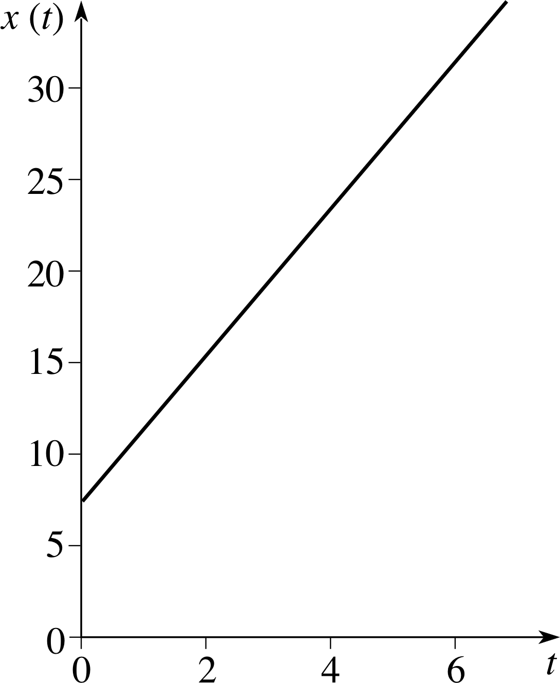
Figure 26 See Answer T6.
Answer T6
The graph of x (t) = 4t + 7 is shown in Figure 26.
A note on mathematical terminology i The set of allowed values for the independent variable of a function is called the domain of the function. Another set called the codomain contains all of the allowed values of the dependent variable (and possibly some other values besides). The formal definition of a function requires that the rule which defines the function should be applicable to each value within its domain and that corresponding to each such value there should be a single value in the codomain.
It is easy to discuss linear motion in terms of functions. For instance, suppose an object is moving along the x–axis of a coordinate system with constant velocity ux. If we let t represent the time that has elapsed since the object passed through the origin, we can say that the position x of the object is a function of the time t and is given by
x (t) = uxt
Similarly, the position of an object that starts from rest at the origin at time t = 0 and moves with constant acceleration ax is given by the function
x (t) = ½ axt2 i
Note that the functions are different in these two cases because the physical circumstances (constant velocity in the first case, constant acceleration in the second) are different. In general we might expect that any particular kind of linear motion will correspond to a particular form for the function x (t).
Now, the process of differentiation has the following purpose:
Given a function x (t), i the process of differentiation can provide a related function x ′(t) such that the value of x ′(t) at any particular value of t is equal to the gradient of the tangent to the graph of x against t at that particular value of t.
The new function x ′(t) produced by the process of differentiation is called the derived function or derivative of x (t) and is usually indicated by the symbol $\dfrac{dx}{dt}$ or, more formally,$\dfrac{dx}{dt}(t)$ to remind us that:
- its value at any particular value of t is equal to the gradient of the graph of x against t at that value of t.
- it is a function of t;
Note that $\dfrac{dx}{dt}$ is not a ratio of two quantities dx and dt, it is a single symbol that represents a particular function. This is why we sometimes write this as $\dfrac{dx}{dt}(t)$.
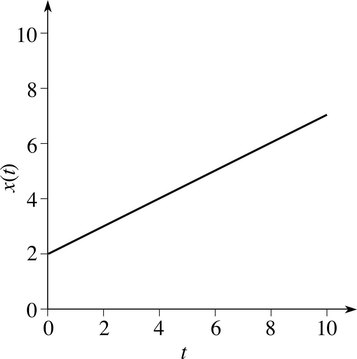
Figure 15 Graphical representation of the function x (t) = 0.5t + 2.
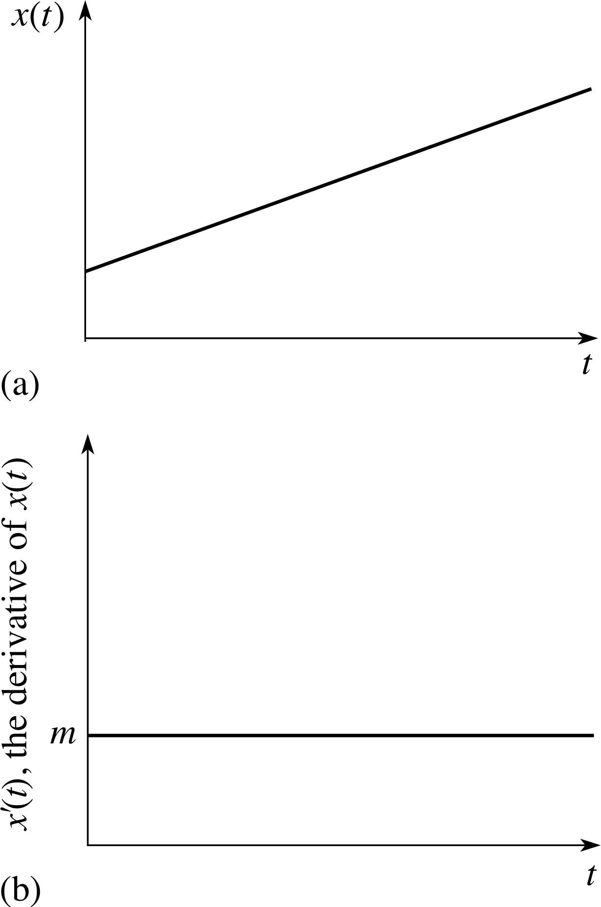
Figure 16 Graphs of (a) x (t) = mt + c and (b) its derivative which is the constant function x ′(t) = m.
3.2 A linear function and its derivative
This subsection uses the algebraic view of a function to calculate derivatives and hence the gradients of graphs of functions. Soon you will be able to dispense with the graphs altogether and calculate derivatives directly.
The most general form of a linear function is x (t) = mt + c, where m and c are constants. The graph of such a function is a straight line of gradient m that intersects the vertical axis at c. Figure 15 shows the graph of x (t) = 0.5t + 2. The gradient of the graph at the point corresponding to t = 2 is 0.5, and it is clear that the gradient has the same value at any other point on the graph. In other words the derivative of x (t) = 0.5t + 2 is 0.5 at t = 2 and at every other value of t. So, in this case, x ′(t) = dx/dt = 0.5 for all values of t.
✦ What is the gradient at the point corresponding to t = 2 on the graph of the function x (t) = mt + c? What is the gradient at all points on the graph? What is the derivative (derived function) of x (t)?
✧ The gradient is m at t = 2 and for all other values of t.
The derivative of x (t) is dx/dt = m for all values of t.
In Figure 15, x and t represented numerical quantities, but if they had represented the position x (in metres) of an object at time t (in seconds), then the gradient of the graph would have represented the velocity vx (in m s−1) of the object. Thus the derivative $\dfrac{dx}{dt}(t)$ describes the velocity at time t.
We can summarize this result in Figure 16 and as follows:
The derivative of the linear function x (t) = mt + c is the constant function which takes the value m everywhere. This corresponds to the result that if the position coordinate, x, increases linearly with time, t, then the velocity vx is constant.
Question T7
The velocity, vx, of an object moving along a straight line is given by the function vx (t) = ux + axt where ux and ax are constants. Find the derivative of vx (t) at t = 2 s. What is the derivative at an arbitrary value of t? In the light of your result interpret the meaning of the constants ax and ux.
Answer T7
Since the graph of vx (t) is a straight line the derivative is the gradient which is ax, not only when t = 2 s but also at all other values of t. So ax, as the notation suggests, is the acceleration. When t = 0, vx = ux, so u is the initial velocity.
3.3 A quadratic function and its derivative
Figure 8 The average velocities plotted on Figure 7 are the gradients of the lines passing through the point corresponding to time t = 5 s.
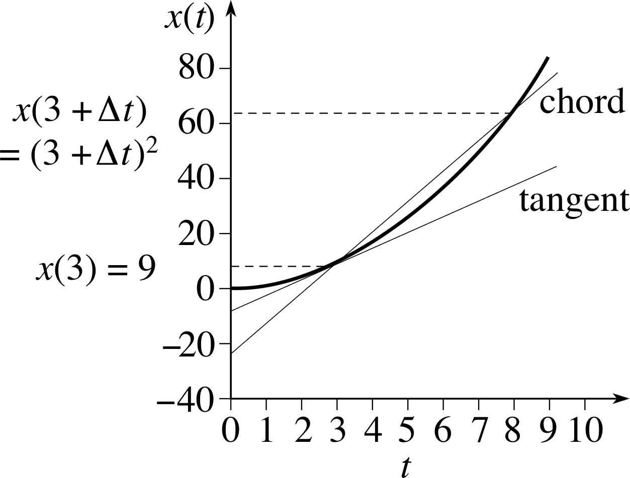
Figure 17 The chord joining the points corresponding to t = 3 and t = 3 + ∆t on the curve x (t) = t2.
Now that you have seen how to differentiate linear functions let us consider quadratic functions. Recall Figure 8 in which we used a sequence of chords i to approximate the tangent to a curve and thus found the gradient of the curve at a point. Let us apply this technique to the differentiation of a simple quadratic function.
Suppose the function we wish to differentiate is x (t) = t2, and suppose we want to find the gradient when t = 3. The corresponding value of x is x (3) = 32. Imagine drawing a chord that cuts the graph of x (t) at t = 3 and cuts it again at another value which we denote t = 3 + ∆t (see Figure 17). i
Since x (t) = t2 the value of x corresponding to t = 3 + ∆t is x = (3 + ∆t)2. The gradient of the chord is therefore
$\text{gradient of chord} = \dfrac{\rm rise}{\rm run}$
$\phantom{\text{gradient of chord}} = \dfrac{(3+\Delta t)^2-3^2}{(3+\Delta t)-3} = \dfrac{9+6\Delta t+(\Delta t)^2-9}{\Delta t}$ i
$\phantom{\text{gradient of chord}} = \dfrac{6\Delta t +(\Delta t)^2}{\Delta t} = 6+\Delta t$
Let us use this expression to calculate the gradients of a sequence of different chords that provide closer and closer approximations to the tangent at t = 3. The chord which intersects the curve at t = 3 and t = 4 has ∆t = 1 and therefore a gradient of 6 + ∆t = 6 + 1 = 7. The gradients of the other chords with smaller ∆t approach the gradient of the tangent as ∆t approaches zero. But the gradient of each chord is given by 6 + ∆t, which approaches 6 as ∆t approaches zero. So 6 is the value for the gradient of the tangent at t = 3. You can demonstrate this for yourself in Question T8.
| t + ∆t | ∆t | Gradient |
|---|---|---|
| 3.5 | 0.5 | 6.5 |
| 3.4 | ... | ... |
| ... | 0.2 | ... |
| ... | ... | 6.01 |
Question T8
Complete Table 4, where the third column is the gradient of the chord joining the points on the curve corresponding to t = 3 and t = (3 + ∆t).
| t + ∆t | ∆t | Gradient |
|---|---|---|
| 3.5 | 0.5 | 6.5 |
| 3.4 | 0.4 | 6.4 |
| 3.2 | 0.2 | 6.2 |
| 3.01 | 0.01 | 6.01 |
Answer T8
The completed Table 4 is given in Table 9. Recall that the gradient is 6 + ∆t.
We can now generalize this process to obtain the gradient at any value of t. Pick a value t and a value close to it denoted by t + ∆t. The corresponding values of x are
x (t) = t2 and x (t + ∆t) = (t + ∆t)2
The gradient of the chord that cuts the graph at t and t + ∆t is given by
${\rm gradient~of~chord} = \dfrac{x(t+\Delta t)-x(t)}{(t+\Delta t)-t} = \dfrac{(t+\Delta t)^2-t^2}{(t+\Delta t)-t}$
$\phantom{{\rm gradient~of~chord} }= \dfrac{t^2+2t(\Delta t)+(\Delta t)^2-t^2}{\Delta t} = 2t+\Delta t$
Now let the chord approach the tangent at t, i.e. let ∆t approach zero. This gives 2t as the gradient at time t. When t = 3 the gradient given by this expression is 6 (= 2 × 3) as we saw before. But we now have a general expression for the gradient at any value of t and hence an expression for the derived function $x^{\prime}(t) = \dfrac{dx}{dt}(t)$.
So, the derivative of a quadratic function x (t) = t2 is $\dfrac{dx}{dt}(t) = 2t$i
Note that the derivative dx/dt = 2t is zero when t = 0 and is negative when t is less than zero. This is exactly what we expect from the gradient of the graph of x (t) = t2 – sketch the graph yourself if you are not convinced.
3.4 Formal definition of a derivative
In the linear and quadratic examples we have investigated so far, we found that at any value of t the derivative dx/dt of a function x (t) is approximated by the gradient ∆x/∆t of a chord. (In this expression ∆x = x (t + ∆t) − x (t) and this represents the change in x in the interval from t to t + ∆t.) We also found that the gradient ∆x/∆t provides an increasingly good approximation to dx/dt as ∆t approaches zero. Indeed, in the limit as ∆t goes to zero it will become exactly equal to the derivative of x (t) at t.
In general, given any function x (t) we define the derivative of x (t) by
$\displaystyle \dfrac{dx}{dt} = \lim_{\Delta t \rightarrow 0}\left(\dfrac{\Delta x}{\Delta t}\right) = \lim_{\Delta t \rightarrow 0}\left[\dfrac{x(t+\Delta t)-x(t)}{\Delta t}\right]$(1)
Note that at any particular value of t, ∆x/∆t is a ratio of two quantities (∆x and ∆t), but dx/dt is not a ratio of dx and dt. Rather you should think of dx/dt at any particular value of t as the value of a function – the derived function x ′(t) – at that value of t.
The definition of the derivative in Equation 1 is subject to the additional proviso ‘if a unique limit exists’. The proviso is necessary because there are some functions that cannot be differentiated at every point in their domain. i Sometimes $\dfrac{dx}{dt}(t)$ is written rather than dx/dt to stress that the derivative is a function.
A mathematical note A precise definition of the limit of an expression as ∆t approaches zero is surprisingly complicated. The limit is an expression that does not involve ∆t but which can be approached as closely as we wish by making ∆t small enough. The complication comes in giving precise meaning to the phrases ‘as closely as we wish ’ and ‘small enough’. In the cases we will meet the limit is obvious. For example, $\displaystyle \lim_{\Delta t\rightarrow 0} (6+\Delta t) = 6$ but there are cases where the limit is much less clear.
Although we are now thinking purely in terms of functions, rather than graphs, the process of finding a derivative looks much the same written down as it did before. For example,
ifx (t) = 4 − 2t + 3t2
thenx (t + ∆t) = 4 − 2 (t + ∆t) + 3 (t + ∆t)2
thus∆x = x (t + ∆t) − x (t) = 4 − 2t − 2 (∆t) + 3t2 + 6t (∆t) + 3 (∆t)2 − (4 − 2t + 3t2) = −2 (∆t) + 6t (∆t) + 3 (∆t)2
Hence∆x/∆t = − 2 + 6t + 3∆t
So$\displaystyle \dfrac{dx}{dt} = \lim_{\Delta t \rightarrow t}\left(\dfrac{\Delta x}{\Delta t}\right) = -2+6t$
Question T9
Find dx/dt for each of the following functions: (a) x (t) = 14 − t (b) x (t) = 1 + t + t2 (c) x (t) = (1 − t)2
Answer T9
(a) x (t) = 14 − t, so x (t + ∆t) = 14 − (t + ∆t).
Thus∆x = x (t + ∆t) − x (t) = 14 − (t + ∆t) − (14 − t) = −t − ∆t + t = −∆t
so$\dfrac{\Delta x}{\Delta t} = \dfrac{-\Delta t}{\Delta t} = -1$
hence$\displaystyle \dfrac{dx}{dt} = \lim_{\Delta t\rightarrow 0}\left(\dfrac{\Delta x}{\Delta t}\right) = -1$
An alternative way of answering is to note that the position–time graph is a straight line with gradient −1.
(b) x (t) = 1 + t + t2
sox (t + ∆t) = 1 + (t + ∆t) + (t + ∆t)2
Thus∆x = ∆t + (t +∆t)2 −t2 = ∆t + t2 + 2t (∆t) + (∆t)2 − t2 = ∆t + 2t (∆t) + (∆t)2
so∆x/∆t = 1 + 2t + (∆t)
hence$\displaystyle \dfrac{dx}{dt} = \lim_{\Delta t\rightarrow 0}\left(\dfrac{\Delta x}{\Delta t}\right) = 1+2t$
(c) x (t) = (1 − t)2 = 1 − 2t + t2
sox (t + ∆t) = 1 − 2 (t + ∆t) + (t + ∆t)2 = 1 − 2t − 2∆t + t2 + 2t∆t + (∆t)2
Thus∆x = −2∆t + 2t∆t + (∆t)2
so∆x/∆t = −2 + 2t + ∆t
hence$\displaystyle \dfrac{dx}{dt} = \lim_{\Delta t\rightarrow 0}\left(\dfrac{\Delta x}{\Delta t}\right) = -2+2t=-2(1-t)$
3.5 Velocity and acceleration as derivatives
In this subsection we will gather together our results concerning derivatives and apply them to position, velocity and acceleration.
Suppose that x (t), vx (t), ax(t) are, respectively, the position, velocity and acceleration of an object at time t as it moves along the x–axis of a coordinate system. i Since velocity is the rate of change of position with respect to time we can write
$v_x(t) = \dfrac{dx}{dt}$ = rate of change of position with respect to time(2)
Similarly, since acceleration is the rate of change of velocity with respect to time
$a_x(t)= \dfrac{dv_x}{dt}$ = rate of change of velocity with respect to time(3)
Thus by two successive differentiations we can go from an expression giving the position to one giving the acceleration. The following questions illustrate this, and also yield some useful general results about differentiation.
Question T10
At time t, the position x of an object moving along a straight line is given by x (t) = p + qt + rt2 where p, q and r are constants. Show that the velocity at time t is vx (t) = q + 2rt.
Answer T10
x (t) = p + qt + rt2, therefore
∆x = x (t + ∆t) − x (t)
∆x = p + q (t + ∆t) + r (t + ∆t)2 − p − qt − rt2
∆x = q∆t + 2rt (∆t) + r (∆t)2
So∆x/∆t = q + 2rt + r∆t
hence$\displaystyle \dfrac{dx}{dt} = \lim_{\Delta t\rightarrow 0}\left(\dfrac{\Delta x}{\Delta t}\right) = q+2rt$
This is the velocity vx.
In order to find the acceleration of this object we must differentiate again.
✦ If vx (t) = q + 2rt find $\dfrac{dv_x}{dt}$.
✧ $\displaystyle \dfrac{dv_x}{dt} = \lim_{\Delta t\rightarrow 0}\left[\dfrac{v_x(t+\Delta t)-v_x(t)}{\Delta t}\right]$
$\displaystyle \phantom{\dfrac{dv_x}{dt} }= \lim_{\Delta t\rightarrow 0}\left[\dfrac{q+2r(t+\Delta t)-q-2rt}{\Delta t}\right]$
$\displaystyle \phantom{\dfrac{dv_x}{dt} }=\lim_{\Delta t\rightarrow 0}\left(\dfrac{2r\Delta t}{\Delta t}\right) = 2r$
Ifx (t) is the quadratic function
x (t) = p + qt + rt2(4)
where p, q and r are constants, then
dx/dt = q + 2rt(5)
and if vx (t) is the linear function
vx (t) = q + 2rt(6) i
then
dvx /dt = ax(t) = 2r(7)
✦ What are the physical interpretations of the constants p, q and r?
✧ If we look at the expressions for x and vx when t = 0, we can see that p must be the initial position x (0) and q must be the initial velocity vx(0). The expression for dvx /dt shows that r is half the (constant) acceleration.
Since r is a constant we have found that a body whose position is a quadratic function of time must be moving with constant acceleration. In fact the converse also holds, and the position is a quadratic function if and only if the acceleration is a constant.
Question T11
If p = −2 m, q = −3 m s−1, r = 1 m s−2 in Equations 4–7, what is t when the velocity is zero?
Answer T11
From Equation 6,
vx (t) = q + 2rt(Eqn 6)
vx (t) = 0 when t = −q/2r = 1.5 s. The initial position, p, does not affect vx.
Finally, we note that when discussing linear motion it is a common practice to describe the location of the moving object in terms of its displacement sx(t) from its initial position x (0). i Thus, rather than basing the discussion on the position x (t), the emphasis is on the difference in positions:
sx(t)= x (t) − x (0)
This has the advantage that when t = 0 we are certain to find sx(0) = 0. Since x (0) is a fixed point it is bound to be true that $\dfrac{ds_x}{dt} = \dfrac{dx}{dt}$, so at any time t the velocity of the moving object will be
$v_x(t)=\dfrac{ds_x}{dt}$ i
Question T12
The motion of an object travelling with constant acceleration ax along the x–axis of a coordinate system is described by the equations
sx(t) = uxt + ½ axt2(8)
vx (t) = ux + axt(9)
where ux is the velocity at time t = 0. Show that Equation 9 is a consequence of Equation 8.
Answer T12
Since $v_x(t) = \dfrac{dx}{dt}$ and s2(t) is a quadratic function it follows from Equations 4 and 5:
x (t) = p + qt + rt2(Eqn 4)
dx/dt = q + 2rt(Eqn 5)
(orby differentiating from first principles as in Question T10) that vx = ux + axt as required.
3.6 Derivatives and rates of change in general
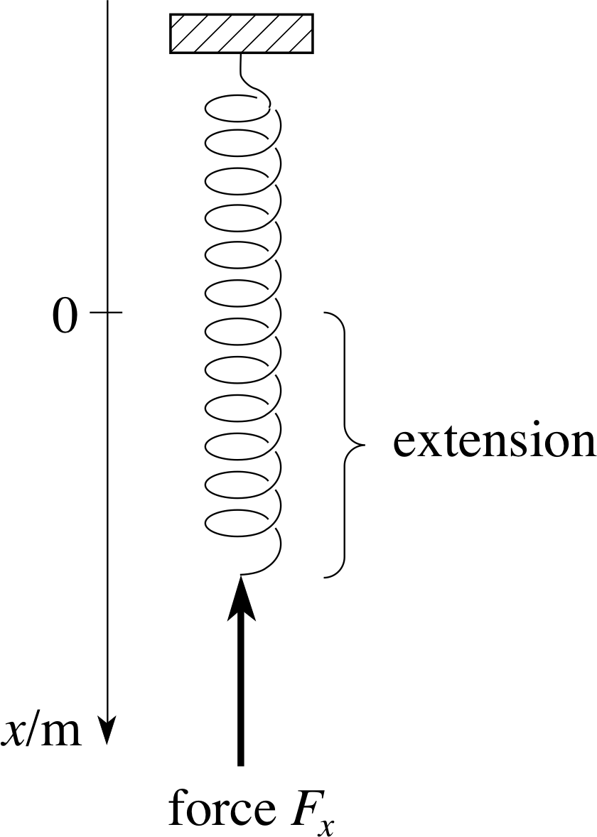
Figure 18 A spring aligned along the x–axis of a coordinate system.
We have seen that both velocity and acceleration are rates of change with respect to time. However ‘rate of change’ is a concept with wider application and does not have to be restricted to change with respect to time. For example, Figure 18 shows a spring aligned along the x–axis of a system of coordinates in such a way that when the spring is extended so that its free end is at x (where x ≥ 0) the force Fx (directed along the negative x–direction) exerted by the spring at its free end is Fx(x) = −kx where k is a constant. (In practice such an expression for Fx(x) might hold true over a limited range of values for x.) If you wanted to know how difficult it would be to increase the extension significantly you might well ask ‘what is the rate of change of the Fx with respect to x?’ In other words, ‘what is the derivative of Fx(x) with respect to x?’
dFx /dx is calculated in the same way as dx/dt – only the letters have changed, not the underlying ideas. Since Fx(x) = −kx is a linear function of gradient k it follows that, dFx /dx = −k. Note that in this case x is the independent variable and Fx is the dependent variable.
Although we have been using x to represent a position coordinate throughout much of this module there is no reason why it should always have that meaning. In fact it is common practice to use the letter x to represent a general independent variable, whilst a general dependent variable is commonly represented by y. (It is in this spirit that we refer to the horizontal and vertical axes of a graph as the x and y axes, respectively.) i
If we adopt this general notation and regard y as a function of x then, irrespective of the particular meaning we attach to x and y, we can define the rate of change of y with respect to x by
$\displaystyle \dfrac{dy}{dx} = \lim_{\Delta t \rightarrow 0}\left(\dfrac{\Delta y}{\Delta x}\right) = \lim_{\Delta t \rightarrow 0}\left[\dfrac{y(x+\Delta x)-y(x)}{\Delta x}\right]$(10) i
Remember that if a unique limit exists for all values of x in the domain of y (x) this procedure defines a function – the derived function y ′(x) – which has the same domain as the original function.
Question T13
Suppose the variation of air temperature, T, with altitude, h, is given by T (h) = ah + b where a and b are constants. Find dT/dh, the rate of change of temperature with respect to altitude. What are the physical interpretations of the constants a and b, and what would be their SI units? (T is measured in kelvin K or degrees Celsius °C.)
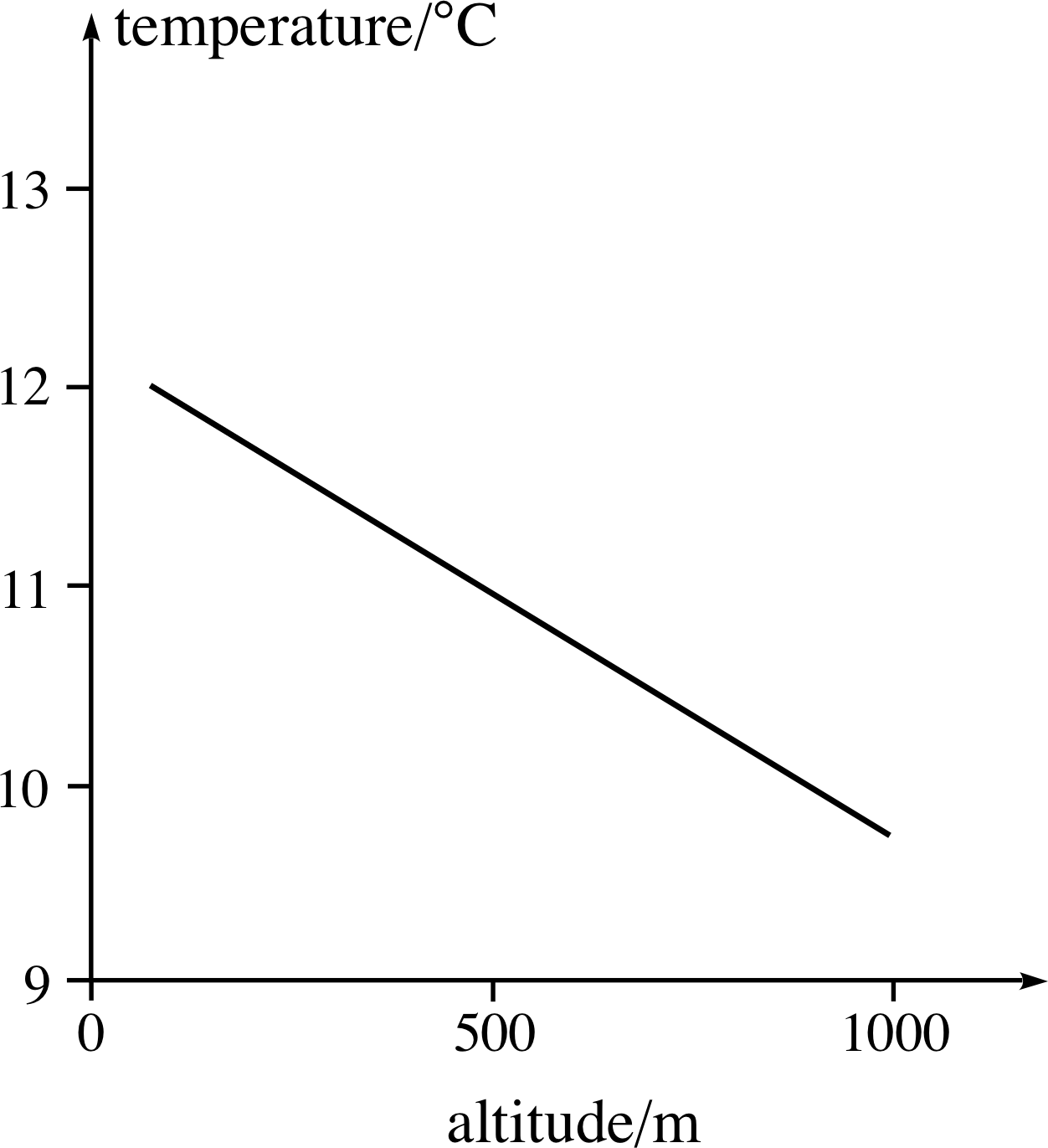
Figure 27 See Answer T13.
Answer T13
The graph of temperature against altitude (Figure 27) is linear so, dT/dh = a. Physically, a is the rate of change of temperature with respect to altitude, and b is the temperature at altitude h = 0. (The choice of where h = 0 is arbitrary, and would generally be taken to be sea level.) The SI units of a would be K m−1 or °C m−1 (since T decreases with increasing altitude, a would have a negative sign) and SI units of b would be K or °C. See Figure 27, which has a gradient of a = −2.5 × 10⁻³ °C m−1.
Question T14
The kinetic energy, Ekin, of a body of mass m moving with speed v is Ekin(v) = ½ mv2. Write down or work out an expression for dEkin/dv and explain its physical meaning.
Answer T14
The function Ekin(v) = ½ mv2 has the same form as the function x (t) = ½ mt2 and comparison with Equations 4 and 5:
x (t) = p + qt + rt2(Eqn 4)
dx/dt = q + 2rt(Eqn 5)
shows that in that case (with p = q = 0 and r = m/2) dx/dt = mt.
SodEkin/dv = mv.
The expression dEkin/dv represents the rate of change of kinetic energy with respect to speed.
4 Conclusion
4.1 The importance of differentiation
Much of physics is concerned with the dynamical processes involved with change and development. Differential calculus is the mathematics of change. It is hardly surprising therefore that many physicists would say that the development of calculus has been the single most important development in mathematics since the time of the ancient Greeks. Nor is it surprising that mastering the techniques of calculus is an important step in the development of every physicist.
In this module we have been mainly concerned with definitions and we have limited our considerations to the differentiation of linear and quadratic functions. In practice physicists rarely have to bother about limits and such mathematical niceties as domains and codomains; they rely on knowing the derivatives of some simple functions and a few basic rules that enable them to differentiate more complicated functions. Armed with this knowledge they are able to use differentiation to tackle an astonishing range of problems that would otherwise be quite intractable. Those wider skills and their applications are the subject of other FLAP modules.
5 Closing items
5.1 Module summary
- 1
-
In linear motion the position of a moving object can be specified by a single position coordinate x at any time t.
- 2
-
The (instantaneous) velocity vx of an object in linear motion is the rate of change of its position coordinate with respect to time.
- 3
-
In linear motion, a plot of x against t is called a position–time graph. The gradient of the tangent to such a graph at any particular value of t determines the (instantaneous) velocity of the moving object at that time. The velocity is constant if and only if the position–time graph is a straight line.
- 4
-
The (instantaneous) acceleration ax of an object in linear motion is the rate of change of its velocity with respect to time.
- 5
-
In linear motion, a plot of vx against t is called a velocity–time graph. The gradient of the tangent to such a graph at any particular value of t determines the (instantaneous) acceleration of the moving object at that time. The acceleration is constant if and only if the velocity–time graph is a straight line.
- 6
-
If a single value of a dependent variable x can be associated with each value of an independent variable t in some specified domain, then we say that x is a function of t, and we speak of the function x (t) (pronounced ‘x of t’).
- 7
-
Given a function x (t), the rate of change of x with respect to t at any particular value of t is given by
$\displaystyle \dfrac{dx}{dt} = \lim_{\Delta t \rightarrow 0}\left(\dfrac{\Delta x}{\Delta t}\right) = \lim_{\Delta t \rightarrow 0}\left[\dfrac{x(t+\Delta t)-x(t)}{\Delta t}\right]$(Eqn 1)
If a unique limit exists for all values of t in some domain, then this formula defines a function called the derivative or derived function, written x ′(t) or $\dfrac{dx}{dt}(t)$.
- 8
-
The value of the derivative dx/dt of a function x (t) at any given value of t is equal to the gradient of the tangent to the graph of x against t at that value of t.
- 9
-
In linear motion, the position coordinate of a moving object may be regarded as a function of time and written x (t). For such an object:
vx (t) = dx/dt = rate of change of position coordinate with respect to time
ax(t) = dvx /dt = rate of change of velocity with respect to time
- 10
-
Generally, if y is a function of x, the derivative dy/dx describes the rate of change of y with respect to x.
If y (x) is the linear function y (x) = ax + b, then dy/dx = a
If y (x) is the quadratic function y (x) = ax2 + bx + c, then dy/dx = 2ax + b
5.2 Achievements
Having completed this module, you should be able to:
- A1
-
Define the terms that are emboldened and flagged in the margins of the module.
- A2
-
Draw position–time and velocity–time graphs.
- A3
-
Understand the relationship between rates of change and gradients of tangents and how they can be approximated by gradients of chords.
- A4
-
Interpret the gradient of a tangent to a position–time or a velocity–time graph as velocity or acceleration, respectively.
- A5
-
Recognize a linear position–time graph as describing constant velocity and a linear velocity–time graph as describing constant acceleration.
- A6
-
Know the definition of a derivative as a limit and give a graphical interpretation of this definiton.
- A7
-
Use the definition of a derivative as a limit to calculate the derivatives of linear and quadratic functions.
- A8
-
Write down an expression for the derivative of a given linear or quadratic function.
- A9
-
Express velocity and acceleration as derivatives for the case of linear motion and solve simple linear motion problems.
- A10
-
Interpret rates of change in terms of the derivative of one quantity with respect to another.
Study comment You may now wish to take the following Exit test for this module which tests these Achievements. If you prefer to study the module further before taking this test then return to the topModule contents to review some of the topics.
5.3 Exit test
Study comment Having completed this module, you should be able to answer the following questions, each of which tests one or more of the Achievements.
Question E1 (A2 and A9)
Sketch roughly the position–time graph of a stone released from rest at a height of 10 m above the ground. Take downwards as the positive x–direction, and note that (neglecting air resistance) such a stone has a constant acceleration ax = 9.8 m s−2. (Take the origin as the initial position of the stone.)
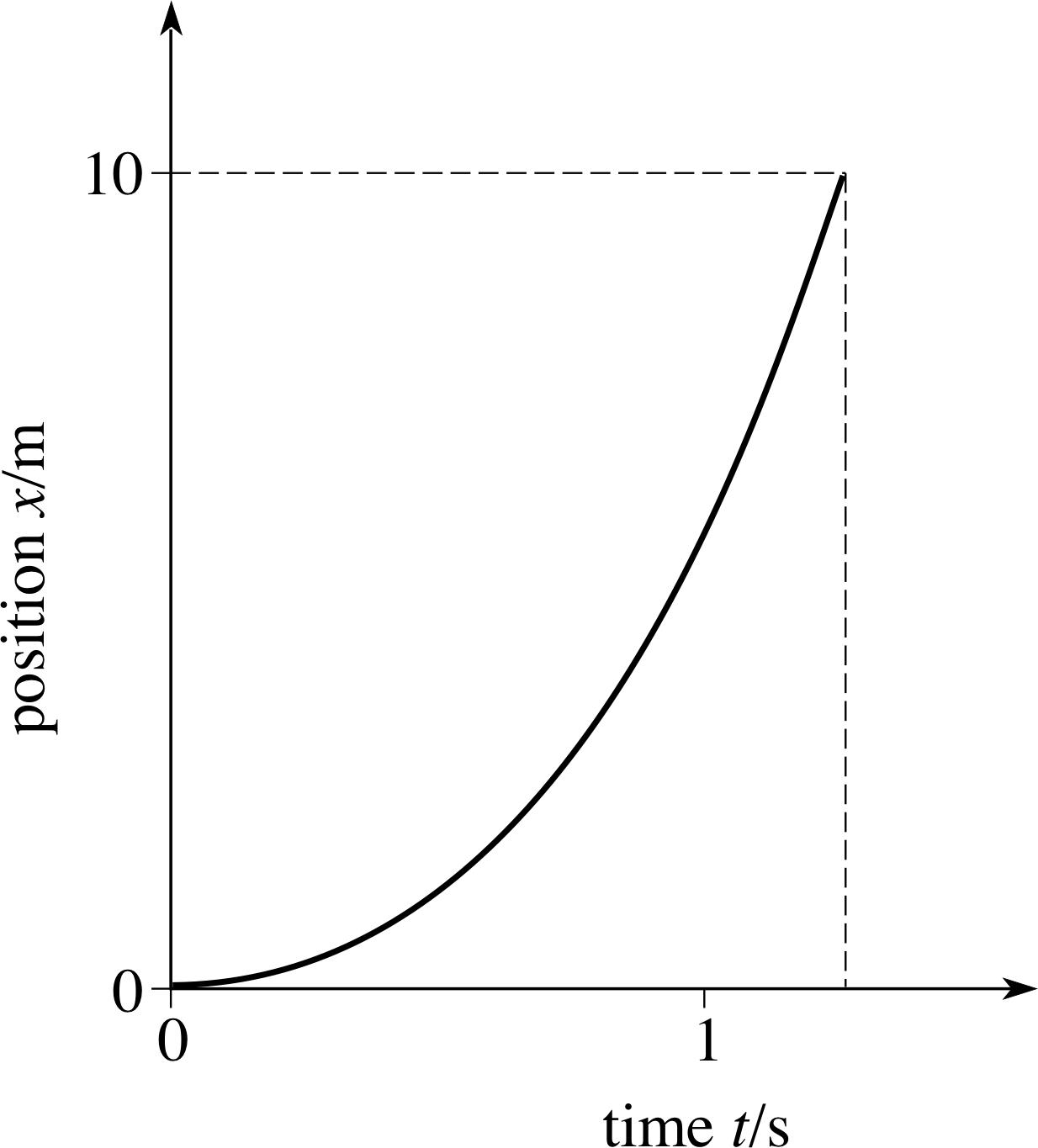
Figure 28 See Answer E1.
Answer E1
From Equation 4,
x (t) = p + qt + rt2(Eqn 4)
with p = q = 0 and r = ax /2 x (t) = axt2/2
The corresponding position–time graph is shown in Figure 28.
(Reread Subsection 2.1Subsections 2.1 and Subsection 3.53.5 if you had difficulty with this question.)
Question E2 (A4)
Figure 19 shows the position–time graph of five different bodies each moving with different constant velocity. If you assume the position and time scales are the same in each case:
(a) Arrange the bodies in order of increasing speed.
(b) Which body has the greatest velocity?
(c) Which body has the least velocity?
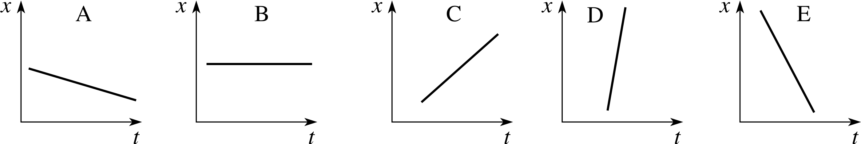
Figure 19 See Question E2.
Answer E2
(a) The steeper the graph, the greater is the change in position in a given interval of time, and therefore the greater is the speed. So in terms of increasing speed the order is B, A, C, E, D.
(b) Graphs C and D have positive gradients (since x increases as t increases). The gradient of D is greater (i.e. more positive) than C, therefore D has the greatest velocity of the five.
(c) Graphs A and E have negative gradients (since x decreases as t increases). The gradient of E is more negative than A, therefore E has the least velocity of the five.
(Reread Subsection 2.2 if you had difficulty with this question.)
| Time/s | Position/m |
|---|---|
| 0.0 | 0.00 |
| 0.1 | 0.05 |
| 0.2 | 0.20 |
| 0.3 | 0.40 |
| 0.4 | 0.80 |
| 0.5 | 1.20 |
| 0.6 | 1.80 |
| 0.7 | 2.40 |
| 0.8 | 3.20 |
Question E3 (A2 and A3)
Table 5 shows position–time measurements of a ball falling from rest under gravity.
(a) Plot the position–time graph.
(b) Using the graph determine the instantaneous velocity at 0.2 s.
(c) Repeat the procedure at 0.6 s.
Figure 29 See Answer E3.
Answer E3
(a) Figure 29 shows the position–time graph, and tangents have been drawn at at 0.2 s and 0.6 s.
(b) Velocity at 0.2 s = gradient at 0.2 s = (1.4 m − 0 m)/(0.8 s − 0.1 s) = (1.4 m)/(0.7 s) = 2 m s−1.
(c) Velocity at 0.6 s = gradient at 0.6 s = (3.0 m − 0 m)/(0.8 s − 0.3 s) = (3.0 m)/(0.5 s) = 6 m s−1.
Comment Note that because the tangent lines are straight their gradients can be found over any chosen interval. We have chosen time intervals from 0.1 s to 0.8 s, and from 0.3 s to 0.8 s in the two cases. The answers are given only to 1 significant figure since it is difficult to read the graph accurately.
(Reread Subsection 2.2 if you had difficulty with this question.)
Question E4 (A2, A3 and A5)
Define the term velocity and explain two methods of obtaining instantaneous velocity from a position–time graph.
Answer E4
Velocity is the rate of change of position. Instantaneous velocity is the gradient of the tangent to the position–time curve at a particular time, and can be obtained by:
(a) drawing the tangent and calculating its gradient.
(b) approximating the tangent by chords, calculating the gradients of the chords and taking the limit as the chords approach the tangent.
(Reread Subsection 2.2Subsections 2.2, Subsection 3.13.1 and Subsection 3.43.4 if you had difficulty with this question.)
Question E5 (A5 and A6)
Write down the definition of the derivative as a limit and use it to find dx/dt when:
(a)x (t) = 3t + 6, (b) x (t) = 6t2 + 4t. i
Answer E5
$\displaystyle \dfrac{dx}{dt} = \lim_{\Delta t \rightarrow 0}\left(\dfrac{\Delta x}{\Delta t}\right) = \lim_{\Delta t \rightarrow 0}\left[\dfrac{x(t+\Delta t)-x(t)}{\Delta t}\right]$
(a) ∆x = x (t + ∆t) − x (t) = 3 (t + ∆t) + 6 − (3t + 6) = 3 (∆t)
So∆x/∆t = 3 and therefore dx/dt = 3.
(b) ∆x = x (t + ∆t) − x (t) = 6 (t + ∆t)2 + 4 (t + ∆t) − (6t2 + 4t) = 12t (∆t) + 6 (∆t)2 + 4 (∆t)
So ∆x/∆t = 12t + 6 ∆t + 4 and therefore dx/dt = 12t + 4.
(Reread Subsection 3.2Subsections 3.2, Subsection 3.33.3 and Subsection 3.43.4 if you had difficulty with this question.)
Question E6 (A7)
Use the formulae for the derivative of linear and quadratic functions to write down the derivatives with respect to t of: i
(a) x (t) = −14 + 7t − 3t2, (b) x (t) = (5t + 7)(2t − 6), (c) x (t) = uxt − ½ gt2 where ux and g are constants.
Answer E6
(a) If x (t) = −14 + 7t − 3t2, then dx/dt = 7 − 6t.
(b) If x (t) = (5t + 7)(2t − 6) = 10t2 − 16t − 42, then dx/dt = 20t −16.
(c) If x (t) = uxt − ½ gt2, where ux and g are constants then dx/dt = ux − gt.
(Reread Subsection 3.2Subsections 3.2, Subsection 3.33.3 and Subsection 3.53.5 if you had difficulty with this question.)
Question E7 (A7 and A8)
If x (t) = p − qt + rt2 find the acceleration at time t = 2 s if p = 13 m, q = 11 m s−1, r = 7 m s−2.
Answer E7
The velocity is vx(t) = dx/dt = −q + 2rt and the acceleration is ax(t) = dvx /dt = 2r = 14 m s−2 for all values of t
(Reread Subsection 3.2Subsections 3.2, Subsection 3.33.3 and Subsection 3.53.5 if you had difficulty with this question.)
Question E8 (A9)
The area, A, of a circle radius r is πr2.
(a) What is meant by dA/dr? Find an expression for dA/dr.
(b) Write down an expression for the difference, D, between the area of a square of side 2r and a circle of radius r.
(c) Find an expression for dD/dr and interpret it.
Answer E8
(a) dA/dr is the rate of change of area with respect to radius. dA/dr = 2πr which shows that the area increases at a rate that is linearly proportional to the radius.
(b) The difference, D, between the area of a square of side 2r and a circle of radius r can be expressed as
D (r) = 4r2 − πr2 = (4 − π)r2
(c) dD/dr = 8r − 2πr = 2 (4 − π)r. This is always positive and increases with increasing r. Hence the difference between these two areas also increases at a rate that is linearly proportional to the radius.
(Reread Subsection 3.5Subsections 3.5 and Subsection 3.63.6 if you had difficulty with this question.)
Study comment This is the final Exit test question. When you have completed the Exit test go back and try the Subsection 1.2Fast track questions if you have not already done so.
If you have completed both the Fast track questions and the Exit test, then you have finished the module and may leave it here.
Study comment Having read the introduction you may feel that you are already familiar with the material covered by this module and that you do not need to study it. If so, try the following Fast track questions. If not, proceed directly to the Subsection 1.3Ready to study? Subsection.