MATH 4.4: Stationary points and graph sketching |
PPLATO @ | |||||
PPLATO / FLAP (Flexible Learning Approach To Physics) |
||||||
|
MATH 4.4: Stationary points and graph sketching
1 Opening items
1.1 Module introduction
1.2 Fast track questions
1.3 Ready to study?
2 Stationary points and the first derivative
2.1 The dinner party problem
2.2 Graphs, gradients and derivatives
2.3 Global maxima and minima
2.4 Local maxima and minima
2.5 The first derivative test
2.6 Exceptional cases
2.7 Back to the dinner party
3 Stationary points and the second derivative
3.1 Graphical significance of the second derivative
3.2 The second derivative test
3.3 Points of inflection
3.4 Which test should you use?
4 Graph sketching
4.1 The value of graph sketching
4.2 A scheme for graph sketching
4.3 Examples
5 Closing items
5.1 Module summary
5.2 Achievements
5.3 Exit test
The watt is the SI unit of power, 1 W = 1 J s−1.
The definitions of function and gradient contained in this subsection are only intended to be brief reminders. You will find more introductory discussions elsewhere in FLAP. See the Glossary for detailed references.
There are some functions for which it is not possible to work out the gradient at every point. These are considered later.
Just as there are some functions that do not have a gradient at every point, so there are some functions that do not have a derivative at every point. These are considered later.
When referring to an interval mathematicians generally have in mind parts of the number line along which all real numbers are sequentially arranged along the horizontal axis of a graph. For this reason they naturally refer to numbers as being to the left or to the right of other numbers according to their respective values. When an interval is defined they also speak of the right–hand and left–hand end of that interval.
Try substituting some specific values of x into $\dfrac{dy}{dx}=1-0.02x$ if you cannot see that this is the case.
Note that a particular global maximum or minimum may occur more than once on a given interval. For instance y = 2x2 over −1 ≤ x ≤ 1, has global maxima of 2 at x = −1 and at x = 1. The constant function y = a attains both its maximum and minimum values at every point in any interval since its maximum and minimum are both equal to a.
Some exceptional cases where turning points are not stationary points will be considered later in Subsection 2.6.
The problem with this method is that of knowing what constitutes ‘nearby points’ without plotting the graph. Using points that are too far from the stationary point can easily lead to misleading answers.
It is the need to select ‘nearby’ numerical values in this way that makes this method less reliable than the alternatives (unless we carry out some additional investigations).
Such investigations may indicate a point of inflection (with horizontal tangent), as described in Subsection 3.3.
Don’t worry if you are not familiar with oscilloscopes.
The arrow symbol (→) can be read as ‘approaches’ or ‘tends to’.
The second derivative of f (x) is the rate of change of the gradient of f (x). Thus, a positive second derivative implies that the function is becoming steeper ‘upwards’.
Some students find it helpful to remember that
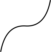
f ′′ (x) > 0 gives a ‘happy’ curve ![]() i.e. concave upwards, while
i.e. concave upwards, while
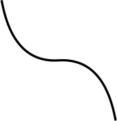
f ′′ (x) < 0 gives a ‘sad’ curve ![]() i.e. concave downwards.
i.e. concave downwards.
We have emphasized this point because it is a common source of errors.
It requires effort to stretch or compress an elastic spring and the potential energy stored in the deformed spring is a measure of this effort. The units of potential energy are joules (J), so the constant K has units J m−2.
It is always a good idea to check your results with the physical meaning if you can. In this case we conclude, from the shape of the graphs near x = L, that deforming the block of rubber by either compressing or stretching it will increase the potential energy, and this is in accord with our physical intuition. Notice that both the ideal model and the realistic model predict this result; however, according to the ideal model it requires a finite amount of energy to compress the rubber to zero length while the realistic model suggests that this would require an infinite amount of energy.
Notice particularly that we require the second derivative to change sign; it is not sufficient for the second derivative to be zero at the point.
It is important to note that just because a section of a graph is concave upwards (or downwards) it does not mean it will have a minimum (or maximum).
A real number is one which is not complex, and does not involve $i = \sqrt{-1\os}$.
Complex numbers are discussed elsewhere in FLAP. See the Glossary for details.
Remember that here we are using the convention that square roots are positive so that $\sqrt{x^2} = \vert\,x\,\vert$
While it is true that the second derivative changes sign as x increases through the value 1, this point is not a candidate for a point of inflection since the function is undefined there. However, we can conclude that the graph changes from concave downwards to concave upwards at this point.
Try some large positive and negative values for x/ex on your calculator.
The volume of a circular cylinder of radius r and height h is πr2h. The area of the curved surface of such a cylinder is 2πrh.
1 Opening items
1.1 Module introduction
The temperature in any week rises and falls each day. Given appropriate equipment you could easily record the temperature at various times during a typical week and plot a graph to show the variation. If you did so, you could then answer a question such as ‘what was the lowest temperature on Wednesday?’ But you could also answer more general questions about the week’s readings such as ‘What was the lowest temperature recorded at any time?’ Both these questions seek minimum values of the temperature; the question about Wednesday is seeking a relative or local minimum, the question about the whole week is seeking an absolute or global minimum.
This module is mainly concerned with the problem of identifying and locating maxima and minima using the techniques of differentiation. It presumes that you have been given physical information in the form of a function, y = f (x) say, and that you have to determine the salient features of that function, particularly the location of its maxima and minima. Problems of this kind are common in physics. For example, you might well be asked to find any of the following:
- The angle at which a projectile should be launched to ensure that it travels as high as possible for a given launch speed.
- The separation between two atoms that will minimize the energy arising from their mutual interaction.
- The lowest temperature on a metal rod that is heated at both ends.
Subsection 2.1 of this module poses a practical problem of this sort; that of providing maximum illumination at a given point on a dining table. The mathematical description of the illumination, using graphs and derivatives, is considered in Subsection 2.2, which also reviews some of the basic concepts needed later. Subsection 2.3Subsections 2.3 and Subsection 2.42.4 explain what we mean by the maxima and minima (both global and local) of a function and explains their relationship to the stationary points at which the function’s first derivative is zero. Subsection 2.5 describes the first derivative test, which is often the simplest way to identify and locate local maxima and minima. Another test, which may be even easier to use in some situations – the second derivative test – is considered in Subsection 3.2. Other aspects of the second derivative of a function, particularly its general graphical significance and the nature of points of inflection at which it changes sign, are considered in Subsection 3.3. The module ends with a discussion of graph sketching in Section 4 which shows how a knowledge of the stationary points and other major features of a function can help you to draw its graph.
Study comment Having read the introduction you may feel that you are already familiar with the material covered by this module and that you do not need to study it. If so, try the following Fast track questions. If not, proceed directly to the Subsection 1.3Ready to study? Subsection.
1.2 Fast track questions
Study comment Can you answer the following Fast track questions? If you answer the questions successfully you need only glance through the module before looking at the Subsection 5.1Module summary and the Subsection 5.2Achievements. If you are sure that you can meet each of these achievements, try the Subsection 5.3Exit test. If you have difficulty with only one or two of the questions you should follow the guidance given in the answers and read the relevant parts of the module. However, if you have difficulty with more than two of the Exit questions you are strongly advised to study the whole module.
Question F1
Under certain circumstances, when sound travels from one medium to another, the fraction of the incident energy that is transmitted across the interface is given by
$E(r) = \dfrac{4r}{(r+1)^2}$
where r is the ratio of the acoustic resistances of the two media. Find any stationary points of E (r), classify them as local maxima, local minima or points of inflection, and sketch the graph of E (r) for r ≥ 0.
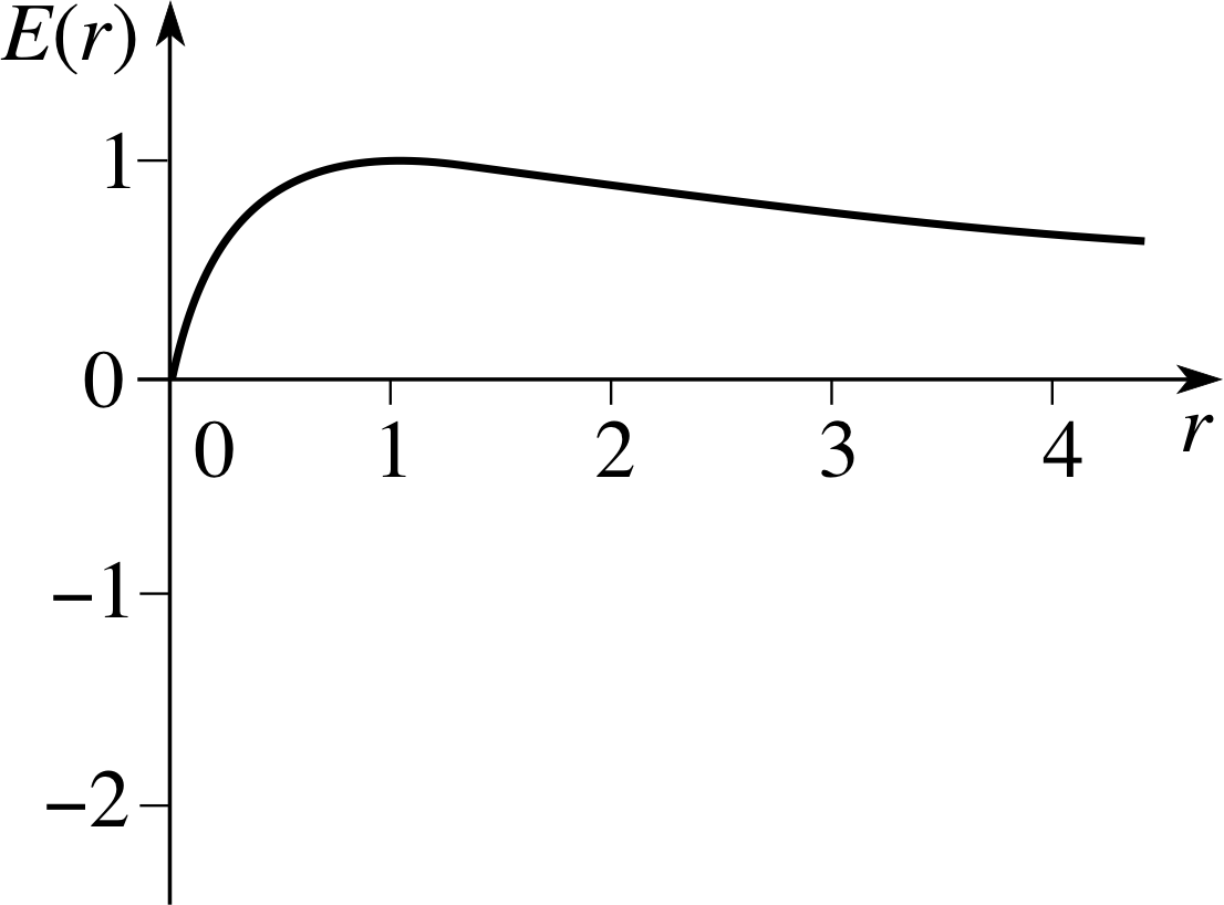
Figure 23 See Answer F1.
Answer F1
Using the quotient_rule_of_differentationquotient rule we find
$E'(r) = \dfrac{(r+1)^2 \times 4 - 2(r+1) \times 4r}{(r+1)^4}$
So,$E'(r) = \dfrac{4-4r}{(r+1)^3} = \dfrac{4(1-r)}{(r+1)^3}$
When r = 1, E ′ (r) = 0.
For r just less than 1, E ′ (r) > 0
For r just greater than 1, E ′ (r) < 0
Hence there is a local maximum at r = 1 and when r = 1, E (r) = 1.
Furthermore, E (0) = 0 and E (r) > 0 for r > 0.
As r → ∞, E (r) → 0.
Figure 23 shows a sketch graph of $E(r) = \dfrac{4r}{(r+1)^2}$.
(There is also a point of inflection for r > 1, but this is not a stationary point.)
Question F2
When air resistance is ignored the horizontal range of a projectile is given by
$R = \dfrac{u^2}{g}\sin(2\theta)$
where u is the initial speed of projection, g is the magnitude of the acceleration due to gravity and θ is the angle (in radians) of projection (with 0 ≤ θ ≤ π/2). Without differentiating the equation, find the value of θ which, for given u, gives the maximum range of the projectile. Confirm that your answer corresponds to a local maximum by investigating the derivatives $\dfrac{dR}{d\theta}$ and $\dfrac{d^2R}{d\theta^2}$.
Answer F2
The maximum value of sin(2θ) is 1 and occurs when 2θ = π/2, i.e. θ = π/4. So, R2 = u2/g.
To confirm that θ = π/4 is a maximum note that:
$\dfrac{dR}{d\theta} = \dfrac{2u^2}{g}\cos(2\theta)$
and that dR/dθ = 0 when θ = π/4. Also note that:
$\dfrac{d^2R}{d\theta^2} = \dfrac{-4u^2}{g}\sin(2\theta)$
So$\dfrac{d^2R}{d\theta^2} \lt 0$ when θ = π/4.
Thus, according to the second derivative test, θ = π/4 is a local maximum.
Question F3
Sketch the graph of the function
$f(x) = x^2+\dfrac{1}{x^2}$ for −3 ≤ x ≤ 3
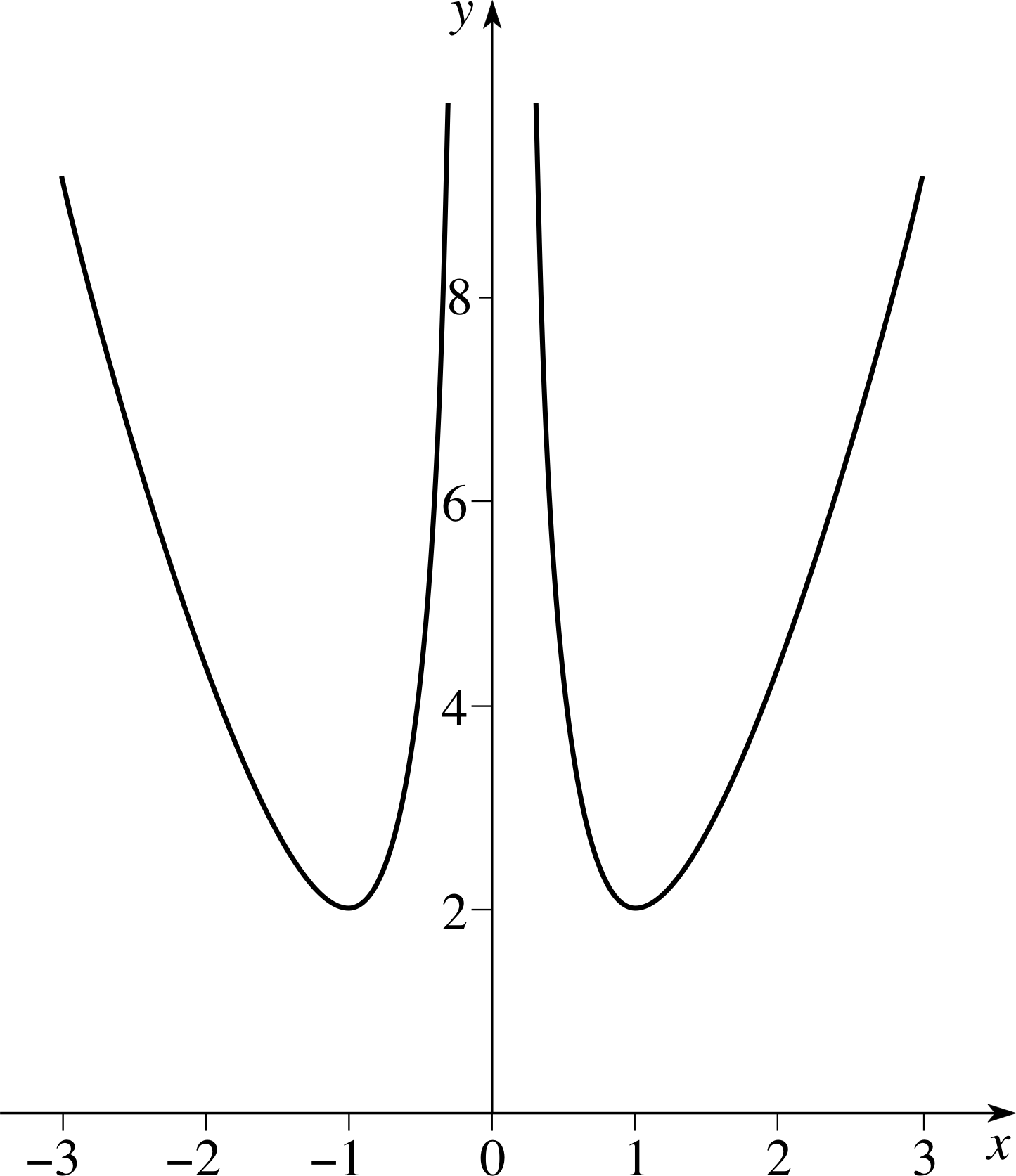
Figure 24 See Answer F3.
Answer F3
f (x) is an even function. It is not defined for x = 0. There is no intercept on either axis. For | x | ≫ 1, f (x) ≈ x2 while for | x | ≪ 1, f (x) ≈ 1/x2.
$f'(x) = 2x - \dfrac{2}{x^3} = \dfrac{2(x^4-1)}{x^3}$
so that f ′ (1) = 0 and f ′ (−1) = 0, and f (1) = 2 and f (−1) = 2.
Also$f''(x) = 2 + \dfrac{6}{x^4}$ so that f ′′ (x) ≥ 0 for x = ±1, and so these points are local minima.
Figure 24 shows a sketch graph of y = f (x).
1.3 Ready to study?
Study comment In order to study this module you should be familiar with the following terms: cosine, derivative, differentiate, domain, exponential function, function, gradient (of a graph), infinity symbol (∞), logarithmic function, inequalityinequality symbols (>, <, ≥, ≤), product_rule_of_differentiationproduct rule, quotient_rule_of_differentiationquotient rule (of differentiation), second derivative, sine, tangent_to_a_curvetangent and variable. In addition you will need to be able to factorize a simple polynomial_expressionpolynomial, solve a quadratic equation and differentiate a range of functions using the techniques of basic differentiation and functions of functions (i.e. composite functions) using the chain rule. If you are unsure of any of these, you can review them now by referring to the Glossary which will indicate where in FLAP they are developed. The following Ready to study questions will help you to establish whether you need to review some of these topics before embarking on the module.
A special note about $\boldsymbol{\sqrt{x\os}}$ Throughout this module we adopt the convention that $\sqrt{x\os}$ is the positive square root of x. Thus, the square roots of x are $\sqrt{x\os}$ and $-\sqrt{x\os}$. It will also be the case that $x^{1/2} = \sqrt{x\os}$.
Question R1
Differentiate the following functions:
(a) f (x) = x4 + 3x2 − 7x + 6, (b) f (x) = sin(2x), (c) $f(x) = \dfrac{3x}{x^2+4}$
(d) $f(x) = \dfrac{2x-5}{\left(x^2+a^2\right)^{1/2}}$, (e) f (x) = x2 ex
Answer R1
(a) Using the sum_rule_for_differentiationsum rule and the constant_multiple_rule_for_differentiationconstant multiple rule of differentiation, we find:
$f'(x) = \dfrac{df}{dx} = 4x^3 + 6x - 7$
(b) Using the chain rule of differentiation, we find:
$f'(x) = \dfrac{df}{dx} = 2\cos(2x)$
(c) Using the quotient_rule_of_differentiationquotient rule of differentiation, we find:
$f'(x) = \dfrac{df}{dx} = \dfrac{3(x^2+ 4) - 3x(2x)}{(x^2+4)^2} = \dfrac{3(4 - x^2)}{(x^2+4)^2}$
(d) f (x) = (2x − 5)(x2 + a2)−1/2
Using the product_rule_of_differentiationproduct rule and the chain rule, we find:
$f'(x) = \dfrac{df}{dx} = 2(x^2+a^2)^{-1/2} - \dfrac12(2x-5)(x^2+a^2)^{-3/2}(2x)$
i.e.$f'(x) = \dfrac{2(x^2+a^2)-(2x^2-5x)}{(x^2+a^2)^{3/2}} = \dfrac{2a^2+5x}{(x^2+a^2)^{3/2}}$
(e) Using the product_rule_of_differentiationproduct rule of differentiation, we find:
$f'(x) = \dfrac{df}{dx} = 2x{\rm e}^x+x^2{\rm e}^x = x(x+2){\rm e}^x$
Consult the relevant terms in the Glossary for further details.
Question R2
Find the second derivative of each of the functions (a) to (c) in Question R1.
Answer R2
The second derivatives are as follows:
(a) 12x2 + 6, (b) −4 sin(2x), (c) $\dfrac{6x(x^2-12)}{(x^2+4)^3}$.
Consult second derivatives in the Glossary for further details.
Question R3
Solve the equation x4 − x3 = 0.
Answer R3
Factorizing the left–hand side of x4 − x2 = 0 we obtain x3(x − 1) = 0 and therefore the roots are x = 0 or x = 1.
Consult factorizing in the Glossary for further details.
2 Stationary points and the first derivative
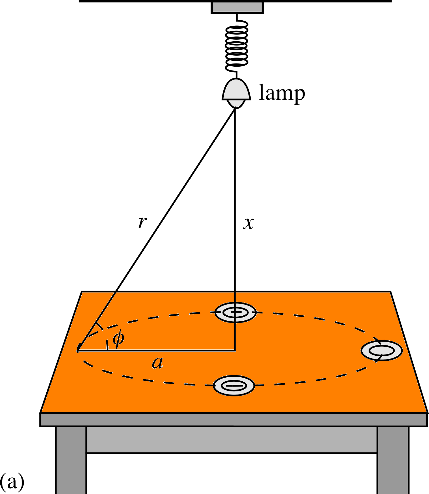
Figure 1 (a) Illuminating a dinner table with a single adjustable lamp
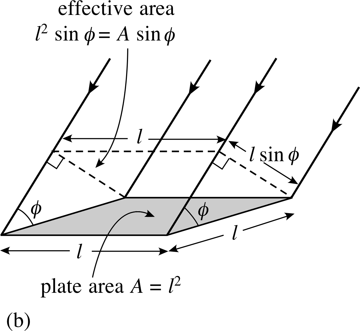
Figure 1 (b) The effective area that a horizontal plate of area A presents to the incident light is A sin ϕ.
2.1 The dinner party problem
Suppose that you and your friends are about to sit down to dinner at a table illuminated by a single lamp suspended at an adjustable height, over the centre of the table (see Figure 1a). One of your friends notes that the plates are poorly lit and asks you to adjust the lamp so that more light falls on them. What would you do? If you lower the lamp you will decrease the distance r between the lamp and the plates which might improve the situation, but you will also reduce the angle ϕ between the light and the plate; so the plates will present a smaller effective area to the light (Figure 1b), and that will make matters worse. Overall, it is not obvious what the effect of lowering the lamp will be. The case is no clearer if you raise the lamp. You will increase r and ϕ and these changes will also produce opposing effects, so again it is unclear whether this will increase the light falling on the plates or not. As a physicist, faced with this dilemma you would probably do what anybody else would do and move the lamp up and down until you had the best result. But as a student of physics you should also appreciate that this simple problem presents an interesting challenge. The experimental fact that there is an optimum position for the lamp shows that there must be a unique solution to the corresponding theoretical problem. The question is, how do you find that solution?
The best way to start looking for this solution is to make sure that the question is clear. Simplified to its bare essentials, the problem can be stated as follows:
Given a horizontal circle of radius a and a lamp that emits energy uniformly in all directions at rate P, at what height x above the centre of the circle must the lamp be located to ensure that the rate at which energy falls on a small horizontal disc of area A, at the perimeter of the circle, is a maximum?
The rate at which energy falls on the disc is given by
$L = \dfrac{PA\sin\phi}{4\pi r^2}$
Note You are not expected to understand the origin of this formula, but A sin ϕ represents the projected area of the disc perpendicular to the incident light, and (P/4πr2) represents the power per unit area in the same plane of projection at a distance of r from the lamp.
The next thing to note is that the only variables on the right–hand side are ϕ and r, and they can both be expressed in terms of x (the height above the centre of the circle) and various constants. From Figure 1 we can see:
$\sin\phi = \dfrac xr$
and$r=\sqrt{x^2+a^2}$
So, if we substitute these two equations into the expression for L we find in turn:
$L = \dfrac{PAx}{4\pi r^3}$
and$L(x) = \dfrac{PAx}{4\pi\left(x^2+a^2\right)^{3/2}}$(1)
where we have replaced L by L (x) to emphasize that the value of L depends on the single variable x, i.e. L is a function of x.
The original physical problem has now been reduced to a mathematical problem involving Equation 1:
Given the values of P, A and a, find the value of x at which L (x) is a maximum.
Solving problems of this general kind is the central theme of this module. In particular we will concentrate on using the techniques of differentiation to investigate functions such as L (x), and to determine the locations of their maxima, minima and any other points of special interest. The solution of the ‘dinner party problem’ that has been posed above will be considered from various perspectives at different points in this section.
2.2 Graphs, gradients and derivatives
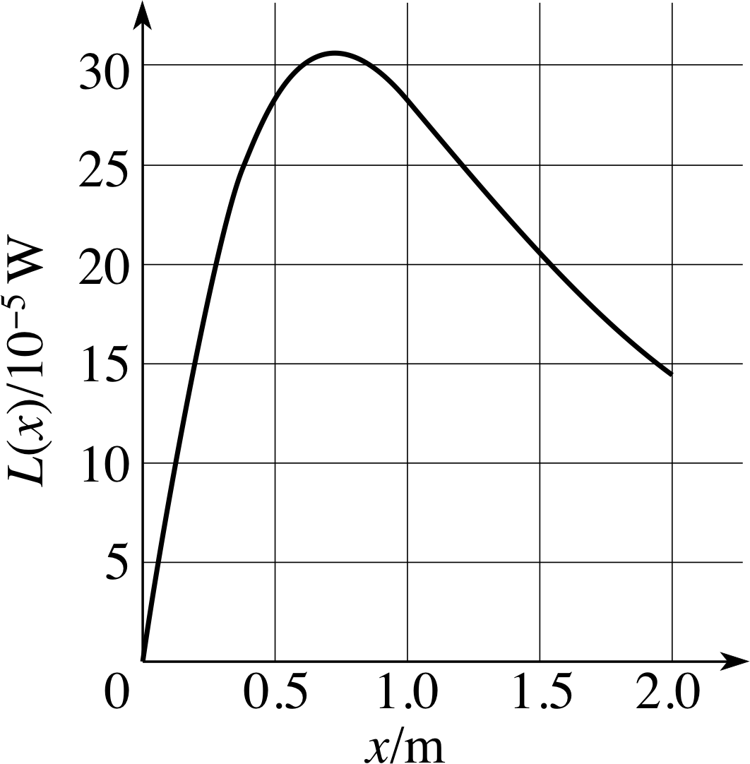
Figure 2 The graph of L (x) for particular choices of P, A and a.
One way of solving the dinner party problem is to plot the graph of L (x) and then determine the optimum value of x. Such a graph is shown in Figure 2 for the case P = 100 W i, A = 1 × 10⁻⁴ m2 and a = 1 m. As you can see, L (x) is a maximum when x is about 0.7 m. This method works, but it is slow, and it can be very inaccurate unless the graph is plotted with care. Furthermore, it requires specific values for the various constants. It would be much better if we could find a non–graphical technique for determining the location of the maximum – especially if that technique were to give an algebraic answer that remained true whatever the values of P, A and a.
The key to developing such a non–graphical (i.e. algebraic) technique lies in recognizing that the gradient (or slope) of a graph provides valuable insight into the behaviour of the graph and of the function that it represents.
Formally, a function f is a rule that assigns a value f (x) in a set called the codomain to each value of x that belongs to a set called the domain of the function. i
In practice, functions are often defined by formulae such as f (x) = 1/(x − 1) and we assume, unless told otherwise, that the domain of the function consists of all those values of x for which the definition makes sense, in this case all real values of x other than 1. We often write y = f (x) so that y = 1/(x − 1) in this case, and we then call x the independent variable and y the dependent variable.
The graph of a function is a plot of the points (x, f (x)). Like Figure 2, such graphs may contain regions where the value of the function increases as x increases or regions where it decreases as x increases. In those regions where its value increases, f (x) is said to be an increasing function and in those regions where it decreases it is said to be a decreasing function.
Given the graph of a function y = f (x), it is usually possible to work out the gradient at any point on that graph. i The gradient provides a measure of the steepness of the graph at a point, i.e. the rate at which y changes in response to a given change in x.
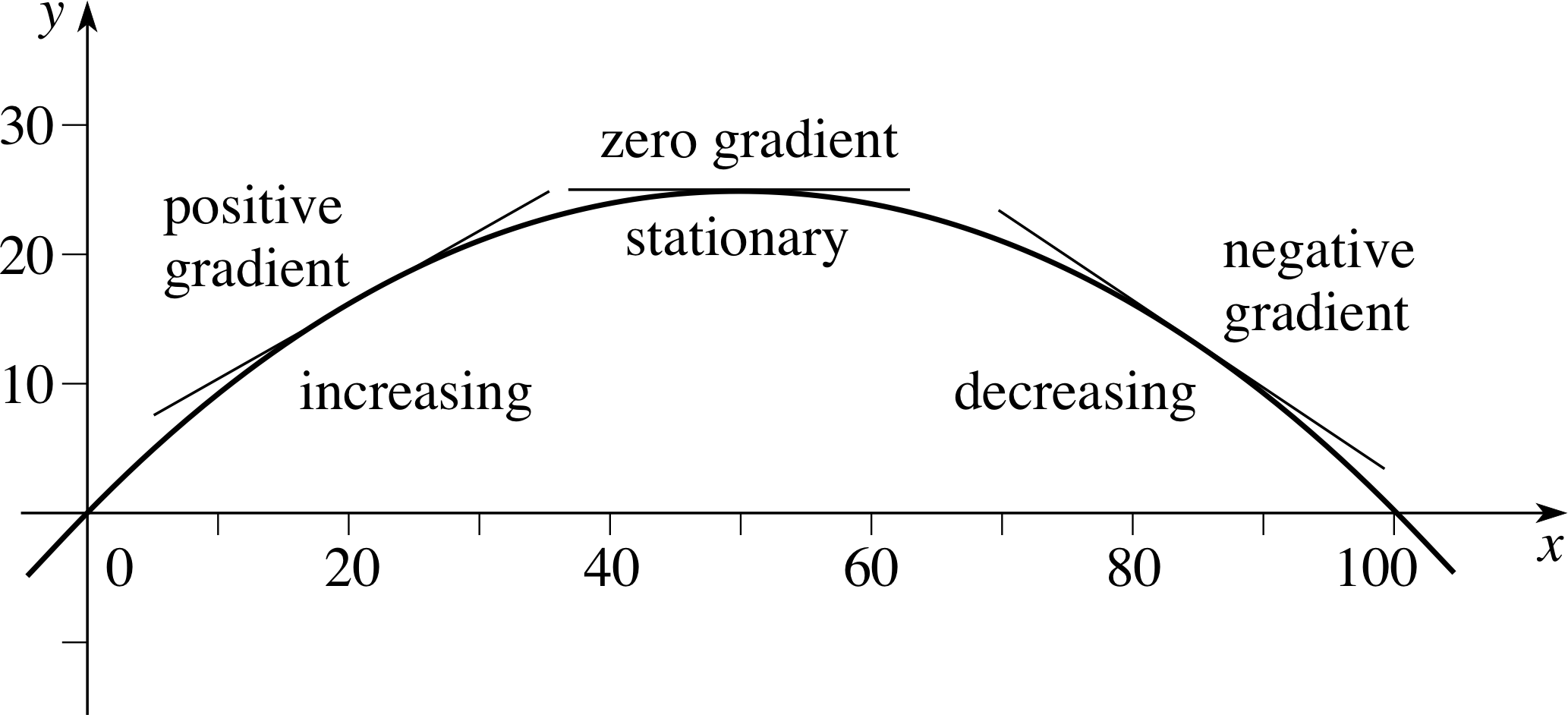
Figure 3 The gradient of y = f (x) at various values of x.
As Figure 3 indicates, the gradient at any point on the graph is given by the gradient of the tangent to the graph at that point. If (x1, y1) and (x2, y2) are two points on the tangent they will be separated by a horizontal ‘run’ ∆x = x2 − x1 and by a corresponding vertical ‘rise’ ∆y = y2 − y1, the gradient will then be ∆y/∆x. It should be clear from Figure 3 that the gradient of a graph is positive where the function is increasing and negative where the function is decreasing. It should also be clear that at the point where the function reaches its maximum (or minimum) the tangent is horizontal, so ∆y = 0 and the gradient is zero. As you will see shortly, it is this observation that provides the basis for an algebraic method of locating maxima and minima.
Given a function y = f (x) it is usually possible to find a related function called the derived function or derivative that may be denoted f ′ (x) or $\dfrac{df(x)}{dx}$, or simply $\dfrac{dy}{dx}$. i Your ability to determine derivatives was tested in Subsection 1.3, but what matters here is your ability to interpret derivatives.
In graphical terms the derivative of a function, evaluated at a point is nothing other than the gradient of that function at that point. Thus, given an appropriate interval, i.e. a range of values such as 0 < x < 0.7 or 0.8 ≤ x ≤ 2 we can say that
f (x) is increasing over an interval if $\dfrac{df}{dx} \gt 0$ for all points in that interval i
and
f (x) is decreasing over an interval if $\dfrac{df}{dx} \lt 0$ for all points in that interval.
The special case $\dfrac{df}{dx}= 0$ leads to another definition:
f (x) is stationary at any point where $\dfrac{df}{dx} = 0$, and such points are called stationary points.
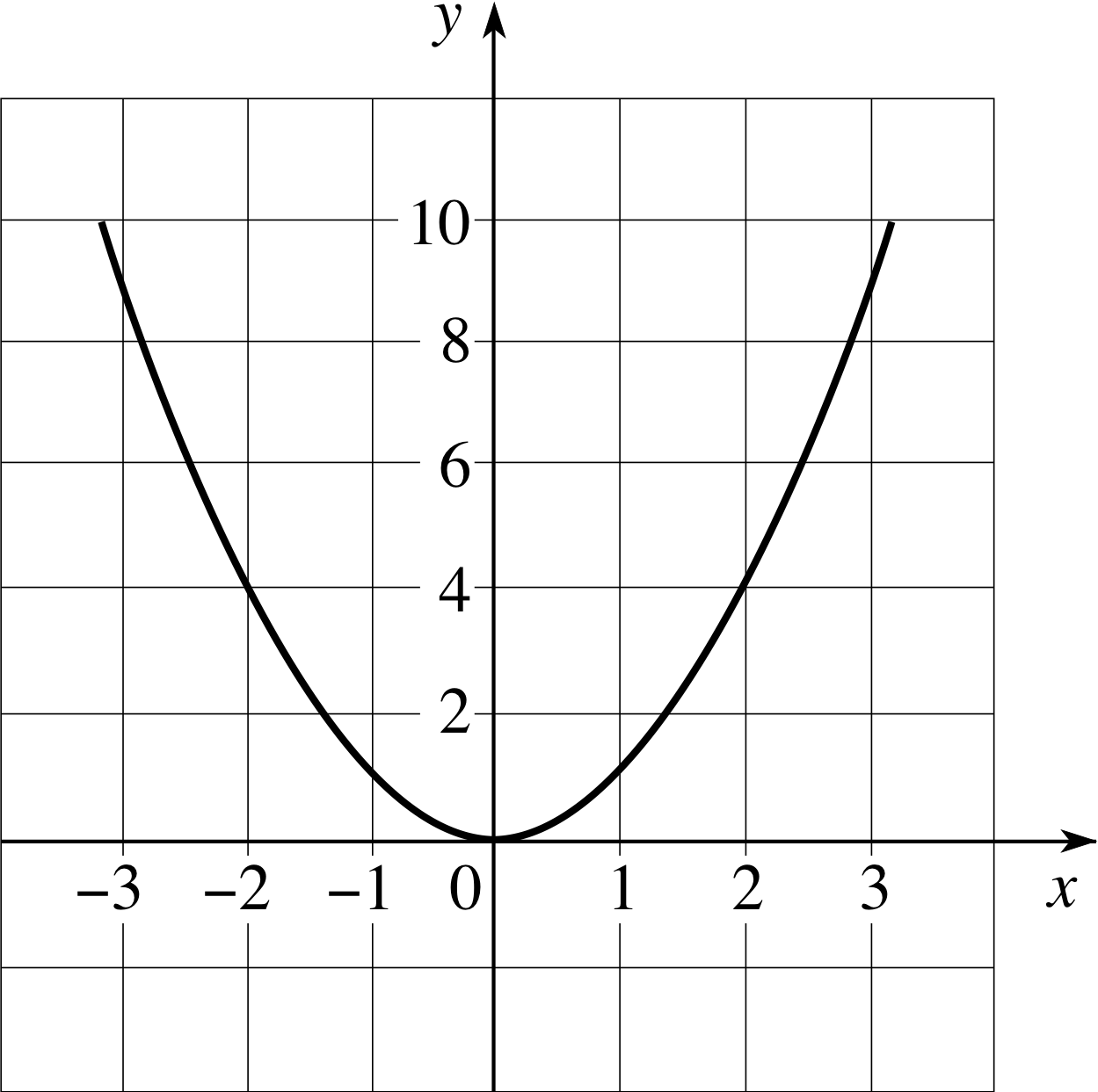
Figure 4 The graph of y = x2 over the interval −3 ≤ x ≤ 3.
✦ How would you describe the behaviour of the function y = x2 (a small section of this graph is shown in Figure 4) in each of the following cases:
(a) 0 < x < 3, (b) −3 < x < 0, (c) when x = 0.
✧ dy/dx = 2x, so:
(a) Over 0 < x < 3, $\dfrac{dy}{dx}$ is positive everywhere so y = x2 is increasing.
(b) Over −3 < x < 0, $\dfrac{dy}{dx}$ is negative everywhere so y = x2 is decreasing.
(c) When x = 0, $\dfrac{dy}{dx}$ is zero. So that y = x2 has a stationary point at x = 0.
(We will have more to say about these points shortly.)
Question T1
By considering their derivatives, determine the intervals over which each of the following functions is increasing, and the intervals over which each is decreasing. What are the stationary points in each case?
(a) f (x) = 6x2 − 3x
(b) g (x) = x2 + 5x + 6
(c) h (x) = 6 + x − 3x2
(d) k (x) = x3 − 6x2 + 9x + 1
(e) $l(x) = 1 + 4x - \dfrac{x^3}{3}$
(f) m (x) = x3
Answer T1
(a) df/dx = 12x − 3. Therefore the function is increasing for x > 1/4, decreasing for x < 1/4, and stationary at x = 1/4.
(b) dg/dx = 2x + 5. Therefore the function is increasing for x > −5/2, decreasing for x < −5/2, and stationary at x = −5/2.
(c) dh/dx = 1 − 6x. Therefore the function is increasing for x < 1/6, decreasing for x > 1/6, and stationary at x = 1/6.
(d) dk/dx = 3x2 − 12x + 9 = 3(x − 3)(x − 1). Since dk/dx < 0 if 1 < x < 3 and dk/dx > 0 if x < 1 or x > 3, it follows that the function is increasing for x < 1 or x > 3, decreasing for 1 < x < 3 and stationary at x = 1 and x = 3.
(e) dl/dx = 4 − x2 = (2 − x)(2 + x). Therefore the function is increasing for −2 < x < 2, decreasing for x < −2 or x > 2, and stationary at x = 2 and x = −2.
(f) dm/dx = 3x2 and it follows that dm/dx > 0 if x ≠ 0 and therefore m (x) is increasing if x > 0 or if x < 0, and it is stationary at x = 0.
2.3 Global maxima and minima
The greatest value of a function in a given interval is known as the global maximum over that interval, and the smallest value of the function in the interval is known as the global minimum. (The equivalent terms absolute maximum and absolute minimum are also widely used.)
Often we wish to determine the global maximum or global minimum of a given function, and the values of the independent variable at which they occur. The simplest case is when the function is either increasing or decreasing throughout the interval, for then the global maximum or minimum must occur at one end of the interval or the other.
✦ Consider the function y = (x − 1)/2 over the interval −4 ≤ x ≤ 4. Where does it take its greatest and least values?
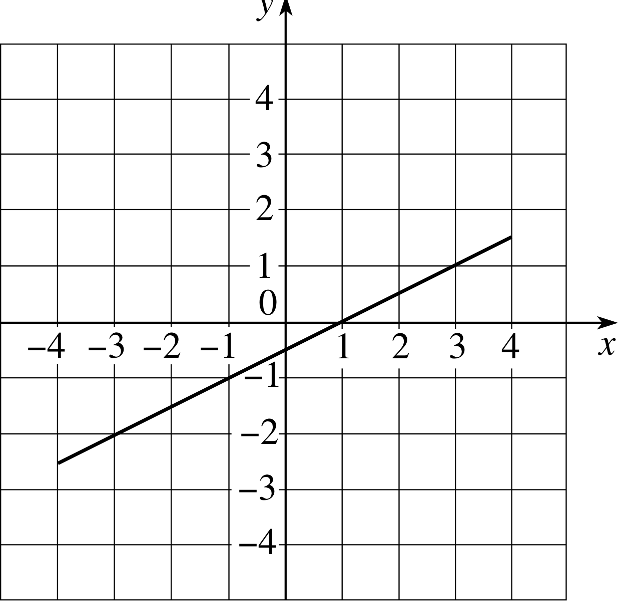
Figure 5 The graph of y = (x − 1)/2.
✧ Differentiating the function, we obtain $\dfrac{dy}{dx} = \dfrac12$. Since this is positive irrespective of the value of x, the function must be increasing throughout the interval. The global minimum of y is −2.5, and occurs when x = −4; the global maximum is 1.5, and occurs when x = 4 (see Figure 5).
Figure 3 The gradient of y = f (x) at various values of x.
In general, an increasing function has its global minimum at the left–hand end of the interval and its global maximum at the right–hand end (and vice versa for a decreasing function).
However, more care is needed when dealing with a function that both increases and decreases in a given interval.
The function y = x − 0.01x2 over the interval 0 ≤ x ≤ 100 is a case in point. (This was the function plotted in Figure 3).
In this case it is clear that the global maximum does not occur at an end of the interval. In fact, from the graph, we can see that the function appears to be increasing for 0 ≤ x < 50 and decreasing for 50 < x ≤ 100, and the global maximum (which turns out to be y = 25) occurs at x = 50. Of course we were fortunate enough in this case to have been given the graph, but we could have managed without it by employing the following strategy.
First we would have differentiated the function y = x − 0.01x2 to obtain
$\dfrac{dy}{dx} = 1 - 0.02x$
then we could have seen that
$\left. \begin{align}\dfrac{dy}{dx} & \gt 0 & & \text{if } 0 \le x \le 50 & & \text{so the function is increasing}\\\dfrac{dy}{dx} & = 0 & & \text{if } x = 0 & & \text{so the function is stationary} \\\dfrac{dy}{dx} & \lt 0 & & \text{if } 0 \lt x \le 100 & & \text{so the function is decreasing} \\\end{align}~~~\right\}$(2) i
Clearly, the stationary point at which dy/dx changes sign corresponds to the global maximum in this case.
✦ Find the global minimum for y = x2 over the interval −3 ≤ x ≤ 3.
Figure 4 The graph of y = x2 over the interval −3 ≤ x ≤ 3.
✧ dy/dx = 2x. So y is decreasing if −3 ≤ x < 0, stationary at x = 0, and increasing if 0 < x ≤ 3. Clearly the global minimum is at x = 0. (The graph of this function was plotted in Figure 4).
It should be clear from the above that finding stationary points can help in locating global maxima and minima but it is important to realize that stationary points are not necessarily maxima or minima. This is demonstrated by the following question.
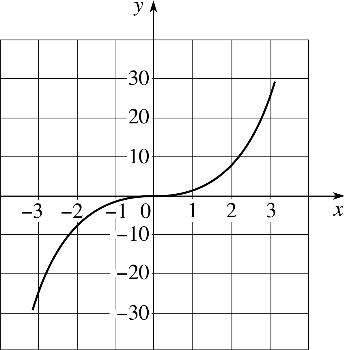
Figure 6 The graph of y = x3.
✦ What are the stationary points of the function y = x3 over the interval−3 ≤ x ≤ 3? What are the global maximum and minimum values on this interval and where are they located?
Figure 6 The graph of y = x3.
✧ First we differentiate the function to obtain $\dfrac{dy}{dx} = 3x^2$. It follows that $\dfrac{dy}{dx}= 0$ when x = 0 so this is the only stationary point (see Figure 6).
However, the function is increasing everywhere else in the interval, so the global maximum is y = 27 and occurs at x = 3, while the global minimum is y = −27 and occurs at x = −3.
So, although stationary points are important in the process of finding global maxima and minima, they do not automatically determine those maxima and minima. In fact, as long as the derivative exists, a general procedure that always works is as follows:
A strategy for finding the global maximum or minimum over an interval
- 1
-
Given a function y = f (x) over an interval, first differentiate to obtain the derivative dy/dx = f ′ (x); then determine the stationary points by finding the values of x for which f ′ (x) = 0.
- 2
-
Calculate the values of f (x) at the stationary points that lie in the interval, and then calculate the values of f (x) at the ends of the interval.
- 3
-
The greatest of these calculated values is the global maximum, the least is the global minimum. i)
You can use this strategy to solve the next question. Notice that there is no need to consider the graph of the function.
✦ Find the global maximum and the global minimum of the following function:
f (x) = x3 − 4x(3)
over the interval −2 ≤ x ≤ 3.
✧ Differentiating the function we obtain f (x) = 3x2 − 4, so the stationary points occur when 3x2 − 4 = 0 which gives $x = \pm 2/\sqrt{3\os} \approx \pm 1.55$.
Notice that both stationary points lie in the given interval.
The values of the function at the stationary points and at the ends of the intervals are:
$f(-2) = 0,~~f(-2/\sqrt{3\os}) \approx 3.079,~~f(2/\sqrt{3\os}) \approx -3.079,~~f(3) = 15$.
Hence, the global maximum is 15 (occurring at x = 3) and the global minimum is (approximately) −3.079 (occurring at $x = 2/\sqrt{3\os}$).
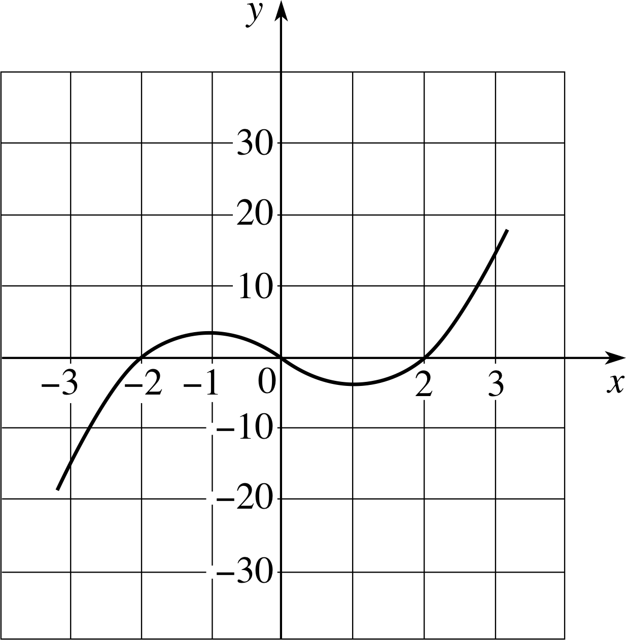
Figure 7 The graph of f (x) = x3 − 4x.
We didn’t need the graph of the function in order to reach the above conclusions, but it is instructive to see what is happening in graphical terms (see Figure 7). As we proceed along the x–axis from −2, the function increases, until we reach $x = 2/\sqrt{3\os}$, it then decreases between $x = -2/\sqrt{3\os}$ and $x = 2/\sqrt{3\os}$, and then increases thereafter.
In the above example both stationary points were in the given interval, but it would not have caused a problem if they had not been; in fact it would have made the process easier, as the following question illustrates.
✦ Find the global maximum and the global minimum values of the following function:
f (x) = x3 − 4x
over the interval 0 ≤ x ≤ 4.
(This is the same function as in the last question, but the interval is different.)
✧ Differentiating the function we find f ′ (x) = 3x2 − 4, so the stationary points are at $x = \pm 2/\sqrt{3\os}$ (as determined above).
Only one of these points $x = 2/\sqrt{3\os}$, lies in the given interval, so we need only calculate the values
$f(0) = 0,~~f(2/\sqrt{3\os})\approx -3.079,~~f(4) = 48$
The global maximum value is 48 (occurring at x = 4), and the global minimum value is (approximately) −3.079 (occurring at$x = 2/\sqrt{3\os}$).
Question T2
Find the global maximum and the global minimum values of the function f (x) = x4 − 4x3 in the interval −1 ≤ x ≤ 4.
Answer T2
If f (x) = x4 − 4x3 then f ′ (x) = 4x3 − 12x2 = 4x2(x − 3). The stationary points occur when x = 0 or x = 3, and both points lie in the interval −1 ≤ x ≤ 4. We consider the values f (−1) = 5, f (0) = 0, f (3) = −27, f (4) = 0 and we see that the global maximum is 5 (occurring at x = −1) while the global minimum is −27 (occurring at x = 3).
Question T3
Find the global maximum and global minimum values of each of the following functions in the intervals given (you should not need to plot the graphs):
(a) f (x) = 4x + 3, (i) in −1 ≤ x ≤ 4 and (ii) in −3 ≤ x ≤ 2.
(b) g (x) = x2 + 4, (i) in −2 ≤ x ≤ 1, (ii) in 2 ≤ x ≤ 5 and (iii) in −3 ≤ x ≤ 2.
(c) h (x) = 4 − (x − 1)2, (i) in 0 ≤ x ≤ 3 and (ii) in 2 ≤ x ≤ 3.
Answer T3
(a) f ′ (x) = 4 which is > 0 and thus the gradient is positive for all x, and f (x) is increasing in any interval.
(i) Over −1 ≤ x ≤ 4 the global minimum value of f (x) is −1 and is attained at x = −1 (the left–hand end of the interval) while the global maximum value, 19, is attained at x = 4 (the right–hand end of the interval).
(ii) Over −3 ≤ x ≤ 2, the global minimum occurs at x = −3 with f (−3) = −9; the global maximum occurs at x = 2 with f (2) = 11.
(b) g ′ (x) = 2x so there is a stationary point at x = 0.
(i) Over −2 ≤ x ≤ 1 we examine the values of the function at the stationary point (which occurs in the interval) and at the ends of the interval to obtain g (−2) = 8, g (0) = 4 and g (1) = 5.
Therefore there is a global minimum at x = 0 with g (0) = 4; a global maximum at x = −2 with g (−2) = 8.
(ii) The derivative is positive over the interval 2 ≤ x ≤ 5 so that g (x) is increasing and therefore takes its global minimum value at the left–hand end of the interval and its global maximum value at the right–hand end. Therefore there is a global minimum at x = 2 with f (2) = 8; a global maximum at x = 5 with f (5) = 29.
(iii) Over −3 ≤ x ≤ 2 we examine the values of the function at the stationary point (which occurs in the interval) and at the ends of the interval to obtain g (−3) = 13, g (0) = 4 and g (2) = 8.
Therefore there is a global minimum at x = 0 with g (0) = 4; a global maximum at x = −3 with g (−3) = 13.
(c) Since h ′ (x) = 2(1 − x) there is a stationary point at x = 1.
(i) Over 0 ≤ x ≤ 3 we evaluate the function at the stationary point (which occurs in the interval) and at the ends of the interval to obtain h (0) = 3, h (1) = 4, and h (3) = 0, so that the global maximum value in the interval is 4, attained at x = 1, while the global minimum value is 0 attained at x = 3.
(ii) In the interval 2 ≤ x 3 we see that h ′ (x) = 2(1 − x) which is < 0 and therefore the function is decreasing. The global maximum value is attained at the left–hand end of the interval value in the interval, i.e. h (2) = 3, while the global minimum value occurs at the right–hand end of the interval, i.e. h (3) = 0.
The strategy that we have developed in this section will work very well for a specific function, such as f (x) = 4x + 3 in a specific interval such as −1 ≤ x ≤ 4, because we can simply compare the sizes of numerical values. However, it is less satisfactory (though still correct) for a function involving parameters, such as that which arose in the dinner party problem
$L(x) = \dfrac{PAx}{4\pi\left(x^2+a^2\right)^{3/2}}$(Eqn 1)
Try comparing the sizes of this function at the ends of the interval 0.5 ≤ x ≤ 3 if you doubt that this is so. We will need to develop some more sophisticated tools in order to deal with such cases.
2.4 Local maxima and minima
Figure 7 The graph of f (x) = x3 − 4x.
In the last subsection we saw that in the interval −2 ≤ x ≤ 3 the function f (x) = x3 − 4x (illustrated in Figure 7) has a global maximum at x = 3. However, if we restrict our attention to the region around the stationary point at $x = -2/\sqrt{3\os}$, then we find that the graph is higher at that value of x than at nearby values of x. At such a point we say that the function has a local maximum. Similarly, at the other stationary point, $x = 2/\sqrt{3\os}$, the graph is lower at that value of x than at nearby values, and at such we say that the function has a local minimum. More formally we say that:
The function f (x) has a local maximum at x = a if for all x near to a we have f (x) < f (a), i.e. f (a) is locally the largest value of f (x).
The function f (x) has a local minimum at x = a if for all x near to a we have f (x) > f (a), i.e. f (a) is locally the smallest value of f (x).
Figure 6 The graph of y = x3.
Local maxima and minima are sometimes referred to as relative maxima and relative minima, and are collectively called local extrema. They mark the points at which the function changes from increasing to decreasing (or vice versa). Points of this kind, at which the derivative changes sign, are known as turning points, so that local extrema and turning points are different names for essentially the same thing. (Local extrema is a plural. A single local maximum or minimum is referred to as a local extremum.)
For smooth functions, whose graphs exhibit no sharp kinks or sudden discontinuous jumps, local extrema are always stationary points at which $\dfrac{df}{dx} = 0$. i However, the converse is not true. It is not the case that all stationary points are local extrema – even in the case of smooth functions. The function y = x3 that we considered in the last section again provides a simple example. It is stationary at x = 0, since $\dfrac{dy}{dx} = 3x^2$ which vanishes (i.e. is equal to zero) at x = 0. Nonetheless, as the graph of y = x3 shows (see Figure 6), there is neither a local maximum nor a local minimum at x = 0.
So, given a function y = f (x), how do we find its local maxima and minima without plotting a graph? There are actually three main methods. In all three methods the first step is the same; differentiate the function, set the derivative equal to zero, and solve the resulting equation, $\dfrac{dy}{dx} = 0$, to find the stationary points.
Once this has been done the next step is to investigate (or ‘test’) the stationary points to see which, if any, are local maxima and which are local minima. This is where the three methods differ. One method uses the behaviour of the first derivative as a test; this is described in the next subsection. Another uses the behaviour of the second derivative; this is described in Section 3. The third method is less useful but simpler in some cases and is described below. The most appropriate method to use in any given situation will depend on the details of the function being investigated.
The most obvious way of testing a stationary point x = a to see if it is a local maximum or a local minimum is to evaluate the function at that point and then to compare this value with the value of the function at nearby points either side of x = a. i If the function has smaller values either side of x = a then x = a is a local maximum. If the values are greater either side of x = a then it is a local minimum. If neither of these conditions is true then the stationary point is neither a local maximum nor a local minimum.
✦ Use the above method to find and classify the stationary points of the following functions:
(a) f (x) = 2x3 + 1, (b) f (x) = x4 − 2, (c) f (x) = −3x2 + 6.
✧ (a) $\dfrac{dy}{dx} = 6x^2$, so the only stationary point is x = 0.
At the stationary point, f (0) = 1.
Immediately to the left, at x = −δ, where δ is a small positive quantity, f (−δ) = −2δ3 + 1 so f (−δ) < f (0); immediately to the right at x = +δ, we have f (+δ) = 2δ3 + 1, so f (+δ) > f (0). Thus the stationary point is neither a maximum nor a minimum.
(b) $\dfrac{dy}{dx} = 4x^3$, so the only stationary point is x = 0.
At the stationary point, f (0) = −2.
Immediately to the left, f (−δ) = δ4 − 2, so f (−δ) > f (0).
Immediately to the right, f (+δ) = δ4 − 2, so f (+δ) > f (0).
Thus, in this case the stationary point is a local minimum.
(c) $\dfrac{dy}{dx} = -6x$, so the only stationary point is x = 0.
At the stationary point, f (0) = 6.
Immediately to the left, f (−δ) = −3δ2 + 6, so f (−δ) < f (0).
Immediately to the right, f (+δ) = −3δ2 + 6, so f (+δ) < f (0).
Thus, in this case the stationary point is a local maximum.
The method we have just used has worked well for the simple cases we have chosen, but it involves quite a lot of work (three function evaluations in each case) and could well have yielded results that were difficult to interpret. The method described in the next subsection is usually quicker and easier.
✦ Returning to the dinner party problem, for the case P = 100 W, A = 1 × 10⁻⁴ m2 and a = 1 m, determine the stationary point of L (x) in the interval 0 ≤ x ≤ 2 m
$L(x) = \dfrac{PAx}{4\pi\left(x^2+a^2\right)^{3/2}}$(Eqn 1)
and confirm that it is a local maximum.
Figure 2 The graph of L (x) for particular choices of P, A and a.
✧ $L(x) = \dfrac{PAx}{4\pi\left(x^2+a^2\right)^{3/2}} = \dfrac{PA}{4\pi}x\left(x^2+a^2\right)^{-3/2}$
So, using the product_rule_of_differentiationproduct rule of differentiation we find
$\dfrac{dL}{dx} = \dfrac{PA}{4\pi}\left(x^2+a^2\right)^{-3/2} + \dfrac{PA}{4\pi}x\dfrac{d}{dx}\left[\left(x^2+a^2\right)^{-3/2}\right]$
using the chain rule (i.e. the function of a function rule) to differentiate the final term
$\dfrac{dL}{dx} = \dfrac{PA}{4\pi}\left(x^2+a^2\right)^{-3/2} -\left(\dfrac32\right) \dfrac{PA}{4\pi}x\left(x^2+a^2\right)^{-5/2}(2x)$
i.e.$\dfrac{dL}{dx} = \dfrac{PA}{4\pi}\left[\dfrac{\left(x^2+a^2\right)-3x^2}{\left(x^2+a^2\right)^{5/2}}\right]$
If we set $\dfrac{dL}{dx}$, we see that the only stationary points are those for which (a2 − 2x2) = 0, i.e. $x=\pm a\sqrt{2\os}$ and only one of these ($x=a\sqrt{2\os}$) is in the given interval. Since a = 1 m, the stationary point is at x = 0.707 m.
In this case it is easier to proceed numerically rather than algebraically, so we will note that at the stationary point
$L(0.707\,{\rm m}) = \dfrac{100\,{\rm W}\times 1\times 10^{-4}\,{\rm m}^2\times 0.707\,{\rm m}}{4\pi\times\left(1.50\,{\rm m}^2\right)^{3/2}} = 3.06\times 10^{-4}\,{\rm W}$
To the left, at x = 0.600 m say, i
$L(0.600\,{\rm m}) = \dfrac{100\,{\rm W}\times 1\times 10^{-4}\,{\rm m}^2\times 0.600\,{\rm m}}{4\pi\times\left(1.36\,{\rm m}^2\right)^{3/2}} = 3.01\times 10^{-4}\,{\rm W}$
To the right, at x = 0.800 m say,
$L(0.800\,{\rm m}) = \dfrac{100\,{\rm W}\times 1\times 10^{-4}\,{\rm m}^2\times 0.800\,{\rm m}}{4\pi\times\left(1.64\,{\rm m}^2\right)^{3/2}} = 3.03\times 10^{-4}\,{\rm W}$
Thus the value of the function is lower either side of the stationary point, so $x=1/\sqrt{2\os}$ m is a local maximum.
(This confirms the approximate result deduced from Figure 2 in Subsection 2.2.)
Figure 7 The graph of f (x) = x3 − 4x.
2.5 The first derivative test
In order to find the stationary points of a function you usually have to differentiate the function and set the resulting first derivative equal to zero. The first derivative test makes further use of the first derivative by using it to determine the nature of the stationary point. In particular it uses the fact, already evident in Figures 3, 4 and 7 that if the first derivative changes sign at a stationary point then that point must be either a local maximum or a local minimum (i.e. a local extremum).
The possible behaviour of the first derivative f ′ (x) in the neighbourhood of a stationary point is analysed more systematically in Table 1.
| Sign of f ′ (x) to left of a |
Sign of f ′ (x) to right of a |
Graphical behaviour |
Conclusion |
|---|---|---|---|
| + | − |  |
The stationary point is a turning point and corresponds to a local maximum |
| − | + |  |
The stationary point is a turning point and corresponds to a local minimum |
| + | + |  |
The stationary point is not a turning point and so the point is not a local extremum |
| − | − |  |
The stationary point is not a turning point and so the point is not a local extremum |
The small graphs given in Table 1 represent the local graphical behaviour of the function. We will have more to say about the last two cases shortly.
For the moment we note the following test.
The first derivative test for local extrema
If f ′ (a) = 0 and f ′ (x) changes sign from positive to negative at x = a, then there is a local maximum at a.
If f ′ (a) = 0 and f ′ (x) changes sign from negative to positive at x = a, then there is a local minimum at a.
If f ′ (a) = 0 but f ′ (x) does not change sign at x = a, then further investigation is required.
(See Subsection 3.2.) i
✦ Find the locations of the local extrema of the function f (x) = x3 − 3x.
Figure 7 The graph of f (x) = x3 − 4x.
✧ We see that f ′ (x) = 3x2 − 3 so that the stationary points occur when 3x2 − 3 = 0, i.e. at x = −1 and x = 1. Factorizing the function, we have f ′ (x) = 3x2 − 3 = 3(x − 1)(x + 1) and we see that the derivative changes sign at x = −1 and x = 1 so that the local extrema occur at these points.
| x | f ′ (x) | Sign of the derivative |
|---|---|---|
| −1.1 | 0.63 | positive |
| −1.0 | 0.00 | sign change |
| −0.9 | −0.57 | negative |
| 0.0 | −3.00 | negative |
| 0.9 | −0.57 | negative |
| 1.0 | 0.00 | sign change |
| 1.1 | 0.63 | positive |
Alternatively we can obtain the same result from a table of values of f ′ (x) (see Table 2).
Notice that we do not need a graph of the function (although it is in fact similar to that of Figure 7).
Question T4
(a) Find the stationary points of the function
f (x) = x3 − 3x2
and decide whether each corresponds to a local maximum, a local minimum or neither.
(b) Find the stationary points of the function
$g(x) = \dfrac{x^3}{3} + 2x^2 +3x+1$
and classify each as a local maximum, a local minimum or neither.
(c) Show that at x = −1 there is a local extremum of the function
h (x) = x4 − 4x3 + 16x
and decide whether it is a local maximum or local minimum. Are there any other local extrema?
[Hint: (x3 − 3x2 + 4) = (x + 1)(x2 − 4x + 4)]
Answer T4
(a) f ′ (x) = 3x2 − 6x = 3x (x − 2) so that x = 0 and x = 2 are stationary points. x = 0 is a turning point which is actually a local maximum since the derivative changes from positive to negative as x passes through 0; x = 2 is also a turning point and a local minimum since the derivative changes from negative to positive as x passes through 2.
(b) g ′ (x) = x2 + 4 x + 3 = (x + 1)(x + 3) so that x = −1, and x = −3 are stationary points. x = −3 is local maximum since the derivative changes from positive to negative as x passes through −3; x = −1 is local minimum since the derivative changes from negative to positive as x passes through −1.
(c) h ′ (x) = 4x3 − 12x2 + 16 = 4(x3 − 3x2 + 4) = 4(x + 1)(x2 − 4x + 4) = 4(x + 1)(x − 2)2
h ′ (−1) = 0, hence x = −1 is a stationary point and by considering h ′ (x) either side of x = −1 we see that x = −1 is a local minimum.
There is also a stationary point at x = 2, but this point is not a turning point, and so cannot be an extremum, since h ′ (x) is positive on each side of x = 2.
2.6 Exceptional cases
Functions that are not differentiable
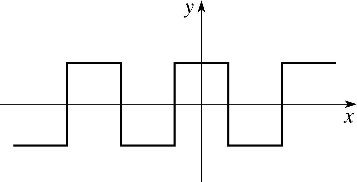
Figure 8 A square wave.
Occasionally you may come across functions that cannot be differentiated at various points; in fact in some situations we go out of our way to construct such functions. The ‘square wave’ and ‘saw-tooth wave’ that are so useful in the control of oscilloscopes i are cases in point (see Figure 8).
The techniques that have been developed in this module require only a minor modification to deal with such cases, as the following example illustrates.
Consider the function f (x) = | x |, which is defined as follows:
$f(x) = \cases{~~x, & \text{for } x \gt 0\\~~0, & \text{for } x = 0\\-x, & \text{for } x\lt 0}$
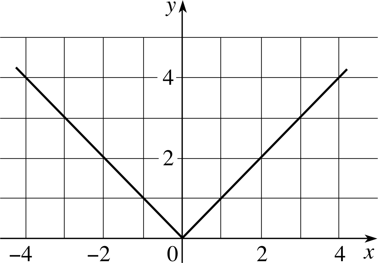
Figure 9 The graph of the function f (x) = | x |.
The derivative f ′ (x) does not exist at x = 0. For x > 0, f ′ (x) = 1 (positive) while for x < 0, f ′ (x) = −1 (negative) so there is no unique value that can be associated with f ′ (x) at x = 0. However, the graph of the function, Figure 9, shows that it has a local minimum at x = 0.
To test (without drawing the graph) the point at which the derivative fails to exist, in order to see if it is a local maximum or local minimum, we simply examine the sign of the gradient on either side of the point as before. This strategy will succeed provided that the graph of the function does not have a ‘jump’ or ‘break’ at the point in question. A function whose graph has no breaks is described as continuous_functioncontinuous.
Similarly we can adapt this method to determine the global maxima and minima. We just include the values of the function at the points where the derivative fails to exist in our list of values to be tested.
Finding the maxima and minima without using calculus
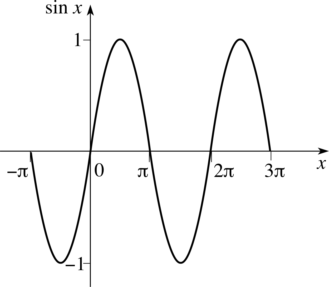
Figure 10 The graph of sin x.
It is not always necessary to use calculus to find the global maximum and minimum values of a function; in fact in some instances it is far easier not to.
For example, suppose that we place no restriction on the values of x, then the greatest and least values of the function y = sin x are 1 and −1 (see Figure 10) and so no calculation is required in order to discover that the greatest and least values of the function y = 1 + sin(2x) are 2 and 0 and that they occur alternately at values of x that are odd integer multiples of π/4.
As another illustration, suppose that a is some positive constant, and that we wish to find the global maximum of the function
$f(x) = \dfrac{1}{\left(x^2 + a^2\right)^2}$
and again we place no restriction on the values of x. We could certainly use the methods that we have developed in this module, but it would involve a little work since we would need to differentiate the function. In fact it is much easier to proceed as follows.
The function attains its greatest value when x2 + a2 is least, i.e. when x = 0. Thus the global maximum value of f (x) is f (0) = 1/a4.
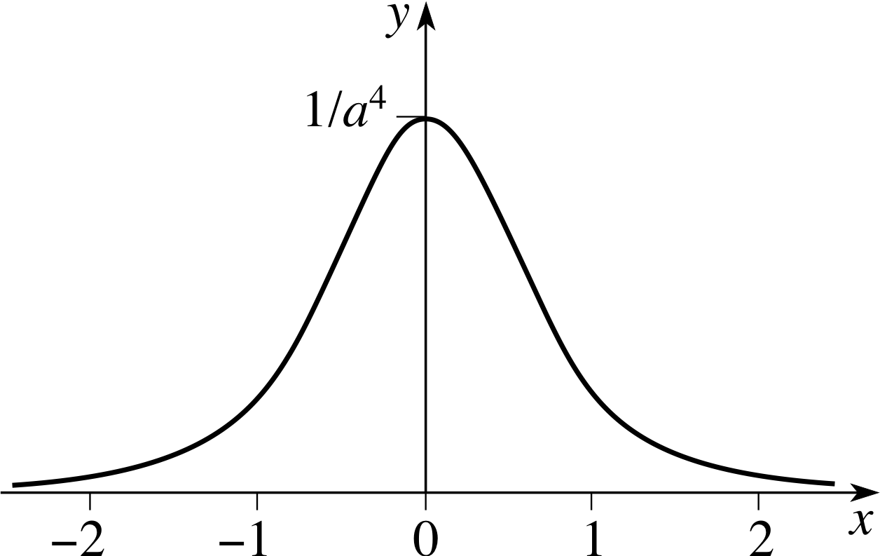
Figure 11 The graph of $y = \dfrac{1}{(x^2+a^2)^2}$.
What would have happened if we had been asked for the global minimum value?
Clearly we want x2 + a2 to be as large as possible; but it has no greatest value since we can make it as large as we please by choosing x sufficiently large. It follows that f (x) may be made as close to zero as we please.
Although the value of f (x) decreases towards zero as x → ±∞, i it never achieves the value of zero and so, strictly, the function does not achieve a global minimum value.
The graph of $y = f(x) = \dfrac{1}{\left(x^2 + a^2\right)^2}$ is shown in Figure 11.
Question T5
Without differentiating the function, use the fact that x2 − 4x + 5 = (x − 2)2 + 1, to find the global maximum value of the function
$f(x) = \dfrac{1}{\left(x^2 - 4x + 5\right)^2}$
in the interval −∞ ≤ x ≤ ∞.
Answer T5
$f(x) = \dfrac{1}{\left[(x-2)^2+1\right]^2}$
As x → ±∞, f (x) → 0, but has no least value. The expression [(x − 2)2+ 1] is least when x = 2 so that f (x) attains its greatest value of 1 when x = 2.
Functions that do not have a global maximum or minimum
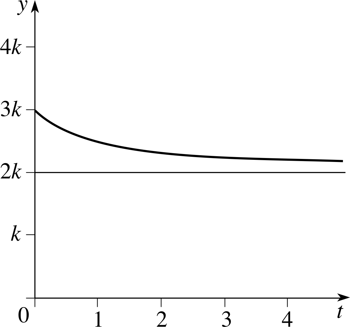
Figure 12 The graph of $y = k\left(\dfrac{2t + 3}{t+1}\right)$.
Not all functions have a global maximum or global minimum in a given region as the above example shows. As an easier example, if we are allowed to choose any real value for x, the function f (x) = x can be as large positive (or negative) as we please and so has no global maximum or minimum value.
Perhaps not quite so obvious is the case of f (x) = 1/x in the interval −1 ≤ x ≤ 1. Here the function is not defined at x = 0, but we can obtain positive or negative values as large as we please by choosing x sufficiently close to 0, and so the function does not achieve a global maximum or minimum.
Some cases are more subtle yet. Suppose, for example, that you are told that the strength of a certain signal is given by $k\left(\dfrac{2t + 3}{t+1}\right)$, where t is some kind of positive numerical variable and k is a positive constant, and that you are asked to find the global minimum value of the signal strength. The graph of the function is shown in Figure 12. For very large values of t, the function value is very nearly equal to 2k, so you might be tempted to give this as your answer. Nonetheless, in strict mathematical terms the function does not have a global minimum and does not achieve the value 2k for any value of t.
2.7 Back to the dinner party
Finally in this section, we return to the dinner party problem from Subsection 2.1. The task was to find the value of x ≥ 0 for which the function
$L(x) = \dfrac{PAx}{4\pi\left(x^2+a^2\right)^{3/2}}$(Eqn 1)
attains its greatest value, where P, A and a are positive constants. We saw earlier that differentiating L (x) gave us
$\dfrac{dL}{dx} = I\dfrac{\left(a^2-2x^2\right)}{\left(x^2+a^2\right)^{5/2}}$
where we have written I = PA/4π, and that the stationary points, given by dL/dx = 0, satisfy x2 = a2/2 so the only meaningful solution is $x = a/\sqrt{2\os}$.
When 0 < x < ($a/\sqrt{2\os}$) we have dL/dx > 0 and when x > ($a/\sqrt{2\os}$) we have dL/dx < 0, so from the first derivative test we see that x = ($a/\sqrt{2\os}$) is a local maximum. In fact we can see more than this, for the function is increasing throughout 0 < x < ($a/\sqrt{2\os}$) and decreasing for all x > ($a/\sqrt{2\os}$). It follows that x = ($a/\sqrt{2\os}$) must actually be a global maximum for all positive values of x.
3 Stationary points and the second derivative
3.1 Graphical significance of the second derivative
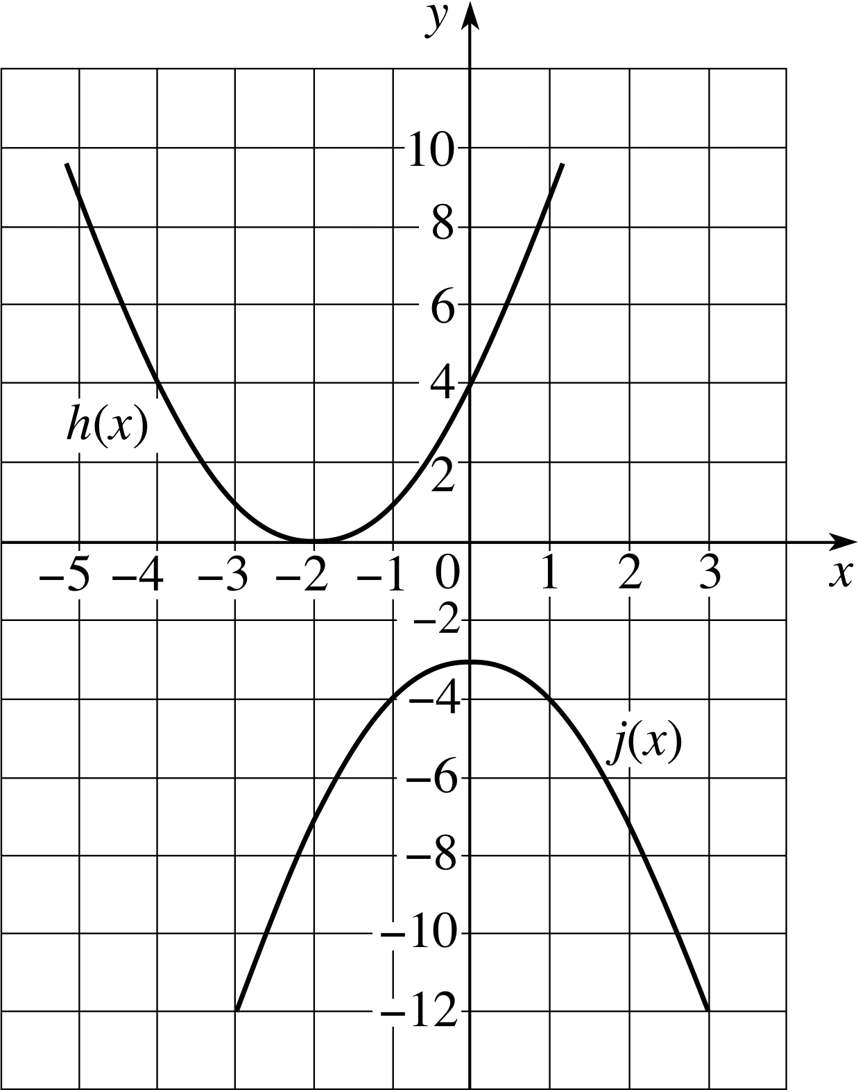
Figure 13 Graphs of functions that are concave upwards (the top graph), and concave downwards (the bottom graph).
Figure 7 The graph of f (x) = x3 − 4x.
Figure 13 shows the graphs of two functions y = h (x) and y = j (x). One might loosely describe the graph of h (x) to be ‘bowl-shaped’ upwards, while the graph of j (x) is ‘bowl-shaped’ downwards.
The technical term for this property of a graph is concavity, and it is closely related to the behaviour of the second derivative of the function, $\dfrac{d^2y}{dx^2}$. i
The first graph is concave upwards, while the second is concave downwards.
It is possible for the graph of a function to be concave upwards on part of its domain and concave downwards elsewhere, for example the graph shown in Figure 7.
You will see shortly that the concept of concavity leads us to another method of classifying local extrema and also to the important notion of a point of inflection.
The concavity of a graph is easily determined from its second derivative as follows:
Let a function f (x) be such that f ′′ (x) is defined for all x in an interval then:
If f ′′ (x) > 0 throughout the interval then the graph of f (x) is concave upwards;
If f ′′ (x) < 0 throughout the interval then the graph of f (x) is concave downwards. i
✦ What is the concavity of the graph of f (x) = x3 + x2?
✧ Differentiating the function we have f ′ (x) = 3x2 + 2x so that f ′′ (x) = 6x + 2. It follows that f ′′ (x) positive if x > −1/3, so the graph is concave upwards, while f ′′ (x) is negative if x < −1/3 and the graph is concave downwards.
Question T6
For each of the following functions use the second derivative to determine the intervals over which the function is concave upwards and the intervals over which it is concave downwards:
(a) f (x) = −x2 + 7x (b) f (x) = −(x + 2)2 + 8 (c) f (x) = −x3 + 6x2 + x − 1 (d) f (x) = (x + 5)3 (e) f (x) = x (x − 4)3 (f) f (x) = x ex
Answer T6
(a) f (x) = −x2 + 7x, f ′ (x) = −2x + 7, f ′′ (x) = −2.
Since f ′′ (x) < 0 the graph of the function is concave downwards everywhere.
(b) f ′ (x) = −2(x + 2), f ′′ (x) = −2.
Since f ′′ (x) < 0 the graph of the function is concave downwards everywhere.
(c) f ′′ (x) = 6(2 − x)
f ′′ (x) > 0 if x < 2, therefore the graph of the function is concave upwards
f ′′ (x) < 0 if x > 2, therefore the graph of the function is concave downwards
(d) f ′′ (x) = 6(x + 5)
f ′′ (x) > 0 if x > −5, therefore the graph of the function is concave upwards
f ′′ (x) < 0 if x < −5, therefore the graph of the function is concave downwards
(e) f ′′ (x) = 12(x − 2)(x − 4)
f ′′ (x) > 0 if x < 2 or x > 4, therefore the graph of the function is concave upwards
f ′′ (x) < 0 if 2 < x < 4, therefore the graph of the function is concave downwards
(f) f ′′ (x) = (x + 2) ex
f ′′ (x) > 0 if x > −2, therefore the graph of the function is concave upwards
f ′′ (x) < 0 if x < −2, therefore the graph of the function is concave downwards
3.2 The second derivative test
At a local minimum the graph of a function is concave upwards while at a local maximum the graph is concave downwards, and this provides us with a useful method known as the second derivative test for classifying local extrema. This method is probably easier to use than the first derivative test, provided that the second derivative is easy to calculate.
The second derivative test for local extrema
If f ′ (a) = 0 and f ′′ (a) < 0, then there is a local maximum at a.
If f ′ (a) = 0 and f ′′ (a) > 0, then there is a local minimum at a.
If f ′ (a) = 0 and f ′′ (a) = 0 then no decision can be made without further investigation. i
✦ The potential energy stored in an ideal_springideal elastic spring of natural length L is given by $V(x) = \dfrac{K(x-L)^2}{2}$ when it is stretched (or compressed) to a length x, where K is a positive constant. i For some real materials, such as a rectangular block of rubber of natural length L, the following model is more accurate
$U(x) = \dfrac K2\left(x^2+\dfrac{2L^3}{x}-3L^2\right)$(4)
where x is again the stretched or compressed length. Find and classify any local extrema of the function U (x).
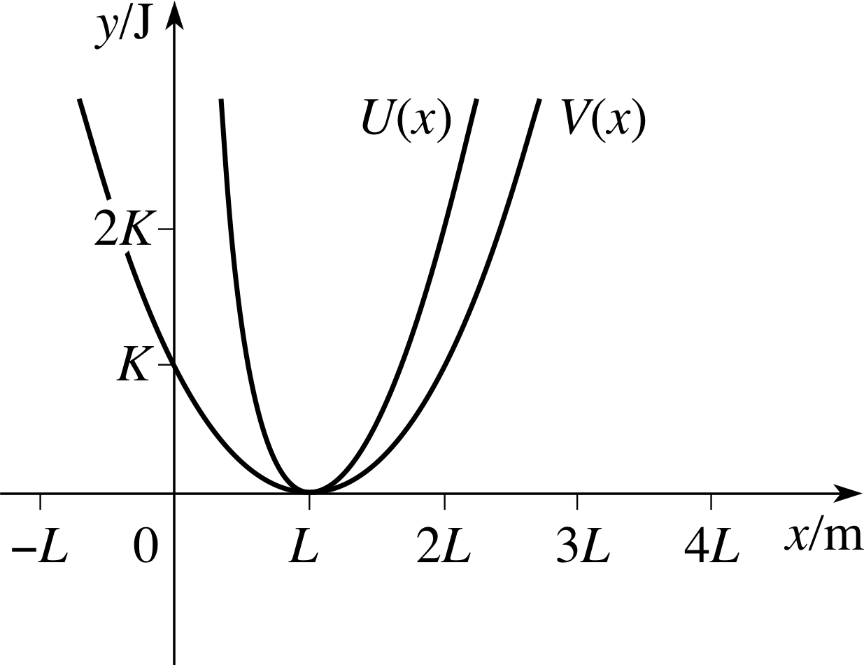
Figure 14 The graphs of y = U (x), the inner curve, and y = V (x), the outer curve.
✧ Differentiating U (x) gives us
$U'(x) = K\left(x - \dfrac{L^3}{x^2}\right)$
Thus, there is a stationary point when x = L.
Now we differentiate again to obtain
$U''(x) = K\left(1 + \dfrac{2L^3}{x^3}\right)$
and we see that U ′′ (L) = 3K, which is greater than zero. It follows from the second derivative test that the function has a local minimum at x = L.
The graphs of U (x) and V (x) are shown in Figure 14. The negative values of x have no physical significance. i
3.3 Points of inflection
A point on a graph where the concavity changes from upwards to downwards or vice versa is called a point of inflection. At a point of inflection the second derivative changes sign. i
✦ Does the function f (x) = x3 − 4x have a point of inflection? If so, where is it?
Figure 7 The graph of f (x) = x3 − 4x.
✧ If f (x) = x3 − 4x then f ′′ (x) = 6x and the second derivative changes sign at x = 0, so that this point is a point of inflection. The function is concave upwards if x > 0 and concave downwards if x < 0 (see Figure 7). i
✦ Does the function f (x) = x4 have a point of inflection? If so, where is it?
Figure 4 The graph of y = x2 over the interval −3 ≤ x ≤ 3.
✧ For the function f (x) = x4 we have f ′′ (x) = 12x2 which is positive for x < 0 and also positive for x > 0. In this case it is certainly true that f ′′ (0) = 0, but the second derivative does not change sign at x = 0, and so there is no point of inflection at x = 0. (In fact this function is positive everywhere except at x = 0 where it is zero, and so has a local minimum at x = 0. The graph is similar in shape to Figure 4 but slightly ‘blunter’ at the origin.)
At a point of inflection, say x = a, the second derivative f ′′ (x) changes sign and so f ′′ (a) = 0. However the condition f ′′ (a) = 0 is not sufficient to ensure that the second derivative changes sign and that a point of inflection exists at x = a.
Note that a point of inflection need not be a stationary point, although it may be. Those points of inflection that are also stationary points (i.e. those at which f ′′ (x) changes sign and f ′ (x) = 0) are called points of inflection with horizontal tangent.
The function f (x) = x3 has a first derivative f ′ (x) = 3x2 and a second derivative f ′′ (x) = 6x, so that the first derivative is zero at x = 0 and the second derivative changes sign there. In this case we have a point of inflection that happens to occur at a stationary point.
In such a case, the fact that the stationary point is not a turning point would be sufficient to tell us that the point is in fact a point of inflection. (See the last two cases in Table 1).
| Sign of f ′ (x) to left of a |
Sign of f ′ (x) to right of a |
Graphical behaviour |
Conclusion |
|---|---|---|---|
| + | − | |
The stationary point is a turning point and corresponds to a local maximum |
| − | + | |
The stationary point is a turning point and corresponds to a local minimum |
| + | + | |
The stationary point is not a turning point and so the point is not a local extremum |
| − | − | |
The stationary point is not a turning point and so the point is not a local extremum |
The function f (x) = x3 − 3x has, as we have seen, a point of inflection at x = 0 but f ′ (x) = 3x2 − 3 is not zero at x = 0.
✦ Does the graph of the potential energy function
$U(x) = \dfrac K2\left(x^2+\dfrac{2L^3}{x}-3L^2\right)$(Eqn 4)
have any points of inflection? (K is a positive constant.)
✧ $U'(x) = K\left(x - \dfrac{L^3}{x^2}\right)\quad\text{and}\quad U''(x) = K\left(1 + \dfrac{2L^3}{x^3}\right)$
so that the second derivative is zero if $\left(1 + \dfrac{2L^3}{x^3}\right) = 0$, i.e. if x3 = −2L3, which gives us
$x=-\sqrt[3]{2\os}L = -2^{1/3}L \approx -1.2599\,L$
We must now check the sign of U ′′ (x) immediately to either side of this value. Since K is a positive constant we have
while U ′′ (−1.2594 L) ≈ −0.0012 K < 0
while U ′′ (−1.2604 L) ≈ +0.0011 K > 0.
and so the second derivative changes sign and there is a point of inflection at x = −21/3L. This mathematical result has no physical meaning for the block of natural rubber since only positive x values (distorted length) are physically acceptable.
Question T7
Find the points of inflection of the following functions
(a) f (x) = −x3 + x2 (b) $f(x) = \dfrac{x^4}{4} - \dfrac{2x^3}{3} + \dfrac{x^2}{2} + 2x$
(c) f (x) = 2x3 − 9x2 + 12x − 4 (d) $f(x) = x^5 - \dfrac53x^3 + 4$ (e) f (x) = sin x (f) $f(x) = x^5 - \dfrac{5x^4}{3}$
Answer T7
(a) f ′′ (x) = 2(1 − 3x). Inflection at x = 1/3 since f ′′ (x) changes sign as x passes through x = 1/3.
(b) f ′′ (x) = 3x2 − 4x + 1 = (3x −1)(x − 1), so that x = 1/3 and x = 1 are points of inflection since f ′′ (x) changes sign as x passes through each of these points.
(c) f ′′ (x) = 6(2x − 3) and x = 3/2 is a point of inflection since f ′′ (x) changes sign as x passes through x = 3/2.
(d) f ′′ (x) = 20x3 − 10x = 10x (2x2 − 1). Points of inflection at x = 0, $x = \pm 1/\sqrt{2\os}$ as f ′′ (x) changes sign as x passes through each of these points.
(e) f ′′ (x) = −sin x. Points of inflection at x = 0, ±π, ±2π, ... since at each of these points f ′′ (x) changes sign.
(f) f ′′ (x) = 20x2(x − 1). Point of inflection at x = 1 because f ′′ (x) changes sign as x passes through the value 1. Also f ′′ (x) = 0 if x = 0 but there is no point of inflection at this point because the second derivative does not change sign.
3.4 Which test should you use?
Given a function y = f (x), which test should you use to determine whether its stationary points are local maxima, local minima or points of inflection? In practice the choice of method is often a matter of taste, but it is sometimes easier to use the first derivative test when the second derivative involves a large calculation.
✦ Examine the function f (x) = 3x5 − 5x3 for local extrema and points of inflection.
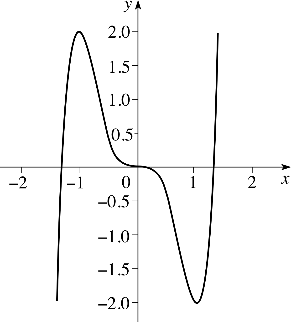
Figure 15 Graph of f (x) = 3x5 − 5x3.
✧ In this case the second derivative is easy to calculate, so differentiating the function, we find
f ′ (x) = 15x4 − 15x2 = 15x2(x2 − 1) and f ′′ (x) = 60x3 − 30x = 30x (2x2 − 1)
Stationary points are located where f ′ (x) = 0, i.e. where 15x2(x2 − 1) = 0, so that x = 0, x = 1 or x = −1.
At x = −1, f ′′ (x) = −30, which is < 0 hence we have a local maximum.
At x = 1, f ′′ (x) = 30, which is > 0 so that we have a local minimum.
At x = 0, f ′′ (x) = 0, so that we cannot come to an immediate conclusion. However f ′′ (x) changes sign at x = 0 so this point must be a point of inflection. (Another indication of this is the presence of a local maximum on one side of x = 0, and a local minimum on the other.)
The second derivative 30x (2x2 − 1) also changes sign at $x=\pm\dfrac{1}{\sqrt{2\os}}$ so that these are two further points of inflection, though neither of them is a stationary point.
Figure 15 shows a sketch of the graph of f (x).
✦ Find and classify the extrema of $f(x) = \sqrt{x^2+1}$.
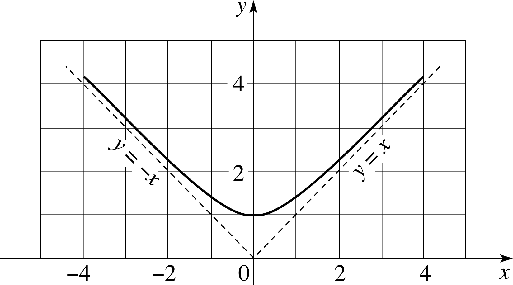
Figure 16 The graph of $f(x) = \dfrac{x}{\sqrt{x^2+1}}$.
✧ Differentiating the function we obtain $f'(x) = \dfrac{x}{\sqrt{x^2+1}}$. In this case it is certainly possible to calculate the second derivative, but the algebra is not pleasant and it is easier to use the first derivative test. First we see that the only stationary point occurs at x = 0, then for x < 0 the derivative is negative while for x > 0 the derivative is positive. It follows that there is a local minimum at x = 0, and this is confirmed by the graph of the function (see Figure 16).
✦ The ‘6–12 function’ is sometimes used to represent the potential energy that arises from the interaction of two atoms separated by a distance r
$U(r) = \dfrac{-A}{r^6} + \dfrac{B}{r^{12}}$
where A and B are positive constants. Left to themselves, the atoms will be at equilibrium when their separation r corresponds to a local minimum of U (r). Find and classify the local extrema of U (r).
Figure 17 The graph of $U(r) = \dfrac{-A}{r^6} + \dfrac{B}{r^{12}}$.
✧ Differentiating the function we have
$U'(r) = \dfrac{6A}{r^7} - \dfrac{12B}{r^{13}} = \dfrac{6}{r^{13}}(Ar^6-2B)$
The derivative is zero if $r = \left(\dfrac{2B}{A}\right)^{1/6}$
The derivative is positive if r is greater, and negative if r is less, than this value; and it follows that there is a local minimum at this point. (The graph is shown in Figure 17).
Question T8
For each of the functions in Question T1 (Subsection 2.2),
(a) f (x) = 6x2 − 3x
(b) g (x) = x2 + 5x + 6
(c) h (x) = 6 + x − 3x2
(d) k (x) = x3 − 6x2 + 9x + 1
(e) $l(x) = 1 + 4x - \dfrac{x^3}{3}$
(f) m (x) = x3
locate the local extrema, and classify them as local maxima or local minima.
Answer T8
(a) f ′ (x) = 12x − 3, f ′′ (x) = 12 > 0. So x = 1/4 is a local minimum.
(b) g ′ (x) = 2x + 5, g ′′ (x) = 2 > 0. So, x = −5/2 is a local minimum.
(c) h ′ (x) = 1 − 6x, h ′′ (x) = −6 < 0. So, x = 1/6 is a local maximum.
(d) k ′ (x) = 3x2 − 12x + 9 = 3(x − 3)(x − 1), k ′′ (x) = 6x − 12
At x = 1 k ′′ (1) = −6 < 0, a local maximum.
At x = 3, k ′′ (3) = 6 > 0, a local minimum.
(e) l ′ (x) = 4 − x2 = (2 − x)(2 + x), l ′′ (x) = −2x
At x = 2, l ′′ (2) = −4 < 0, a local maximum.
At x = −2, l ′′ (−2) = 4 > 0, a local minimum.
(f) m (x) = x2, m ′ (x) = 3x2, m ′′ (x) = 6x
There is a point of inflection at x = 0.
4 Graph sketching
You will have noticed that we have made great use of graphs to illustrate the algebraic results obtained in this module, but the reverse process can be quite productive: we can often use knowledge of local extrema and points of inflection, obtained algebraically, to help us to construct the graph of a function.
4.1 The value of graph sketching
Given a function, for example f (x) = 3x5 − 5x3, we can plot its graph by taking a selection of values for x, calculating the corresponding values of y = 3x5 − 5x3 and drawing a smooth curve through the points (x, y) so generated. With the advent of advanced scientific calculators and graph plotting computer programs, very often the simplest method of producing a graph is to plot it on a machine. However this is not always the case, and it is quite possible that using a machine without some prior knowledge of the graph will be totally unproductive.
You may like to try plotting the graph of the function $f(x) = \dfrac{1}{(10^6 x - 1)(x - 10^6)}$ on a computer, or calculator, if you doubt that this is the case. Another problem that often arises is that of determining the behaviour of a function that involves several algebraic parameters for all values of the parameters rather than for some particular numerical choices.
The purpose of graph sketching, as opposed to graph plotting, is to determine the important features of the graph with the minimum of effort. Of course, if more detailed information is required it will be necessary to carry out further investigation.
4.2 A scheme for graph sketching
Figure 4 The graph of y = x2 over the interval −3 ≤ x ≤ 3.
Figure 6 The graph of y = x3.
In this subsection we present a number of techniques that will produce the required detail for the majority of functions that you are likely to encounter.
1 Symmetry about the y-axis
A function f (x) is said to be even_functioneven if f (−x) = f (x). Examples of even functions are f (x) = 5x2, f (x) = x2n (for any integer n) and f (x) = cos x. The graph of an even function is symmetrical about the y–axis; for an example see the graph of y = x2 in Figure 4.
A function f (x) is said to be odd_functionodd if f (−x) = −f (x). Examples of odd functions are f (x) = 2x, f (x) = x3, f (x) = x2n + 1 (for any integer n), f (x) = sin x and f (x) = tan x.
If f (x) is odd and f (0) is defined then f (−0) = −f (0), i.e. f (0) = −f (0) which implies that f (0) = 0 and therefore the graph of any odd function must pass through the origin. If the portion of the graph for which x ≥ 0 is rotated 180° clockwise about the origin, it coincides with that portion for which x ≤ 0; for an example see Figure 6. Notice that a function may be neither odd nor even. In fact, odd and even functions are rather special cases.
✦ Classify the following functions as odd, even or neither:
(a) f (x) = 3x2 + 2, (b) g (x) = 2x3 − x, (c) h (x) = 3x2 + x.
✧ (a) f (−x) = 3(−x)2 + 2 = 3x2 + 2 = f (x), therefore it is even.
(b) g (−x) = 2(−x)3 − (−x) = −2x3 + x = −g (x), therefore it is odd.
(c) h (−x) = 3(−x)2 + (−x) = 3x2 − x ≠ h (x) or −h (x), therefore it is neither odd nor even.
We notice some special general rules here. All even powers of x are even functions; all odd powers of x are odd functions. Functions which combine odd and even powers of x may or may not have special symmetry. Also the product of two odd functions or two even functions is an even function; the product of an odd and even function is odd.
Question T9
Classify the following functions as odd, even or neither:
(a) x + sin x, (b) x2 − 2 cos x, (c) x2 + sin x, (d) x sin x, (e) x cos x.
Answer T9
(a) Odd, since (−x) + sin(−x) = −(x + sin x)
(b) Even, since (−x)2 − 2 cos(−x) = x2 − 2 cosx
(c) Neither, since (−x)2 + sin(−x) = x2 − sin x
(d) Even, since (−x) sin(−x) = −(−x) sin x = x sin x
(e) Odd, since (−x) cos(−x) = −(x cosx)
2 Forbidden regions
Consider the curve whose equation is
y = (x2 − 1)1/2
In order to obtain a real value for y we require that x2 ≥ 1. i
This means that either x ≥ 1 or x ≤ −1 and there is no part of the curve in the interval −1 < x < 1.
3 Intercepts with the axes
Figure 4 The graph of y = x2 over the interval −3 ≤ x ≤ 3.
Any graph that meets the y–axis does so when x = 0, hence to find such intercepts we simply put x = 0 in the equation.
For example, given y = x3 + 4 we put x = 0 to obtain y = 4.
Similarly, any curve that meets the x–axis does so where y = 0. For the curve whose equation is y = x2(x − 1), putting y = 0 yields x = 0 or x = 1. Such solutions are generally called roots and in this case there may be 4 said to be a double root at x = 0 and a single root at x = 1. Similarly x3(x + 1)2(x − 3) = 0 has a triple root at x = 0, a double root at x = −1, and a single root at x = 3. The single root x = 1 represents a simple crossing point on the axis and the function changes sign there, but at the double root x = 0 the graph touches the x–axis (in a similar fashion to the graph y = x2, Figure 4) and the function does not change sign.
At a triple root the graph would touch the x–axis and change sign y (as in the graph of y = x3, Figure 6). Such roots, corresponding to a factor raised to a power, are often known as multiple roots.
Figure 6 The graph of y = x3.
4 Isolated points where the function is not defined
The function h (x) = 1/x is defined for all values of x except x = 0. In such cases it is often informative to investigate the values of the function immediately above and below the isolated point. Reference to the graph of h (x) in Figure 18 shows that for values of x approaching zero from the positive side, h (x) is large and positive; whereas for values of x approaching zero from the negative side, h (x) is large and negative. A line to which a curve approaches in the limit (as the curve is extrapolated to infinity) but never touches, is called an asymptote. In Figure 18 the line x = 0 may be described as a vertical asymptote and the line y = 0 as a horizontal asymptote.
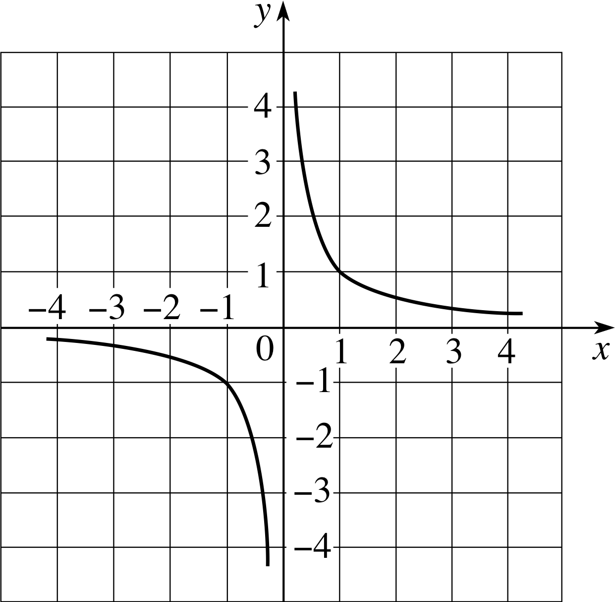
Figure 18 The graph of y = 1/x.
5 Behaviour for large values of | x |
It is sometimes possible to get an idea of a function’s approximate behaviour by ignoring terms in the function that are small in magnitude compared to others.
For example, the function
$f(x) = \sqrt{x^2+1} = \sqrt{x^2}\sqrt{\left(1+\dfrac{1}{x^2}\right)} = \vert\,x\,\vert\sqrt{\left(1+\dfrac{1}{x^2}\right)}$ i
Figure 16 The graph of f (x) = x2 + 1.
can be approximated by g (x) = | x | for values of | x | ≫ 1 because 1/x2 is then much smaller in magnitude than 1. We may write f (x) ≈ | x | as x → ±∞ which means that the function is approximately equal to | x | when x is large (positive or negative). Figure 16 showed the graphs of y = x2 + 1 and y = | x |. In such a case the function f (x) = x2 + 1 is said to approach the function g (x) = | x | asymptotically as x → ±∞.
6 Behaviour for small values of | x |
When x is small and positive, or small and negative, it is sometimes possible to approximate the function by ignoring terms that are small in magnitude. As an example f (x) = x3 − 9x is approximated by the function j (x) = −9x when | x | ≪ 1 because x3 is much smaller in magnitude than −9x. This tells us at once that the tangent to the graph at x = 0 is the line y = −9x.
7 Use of the derivative(s)
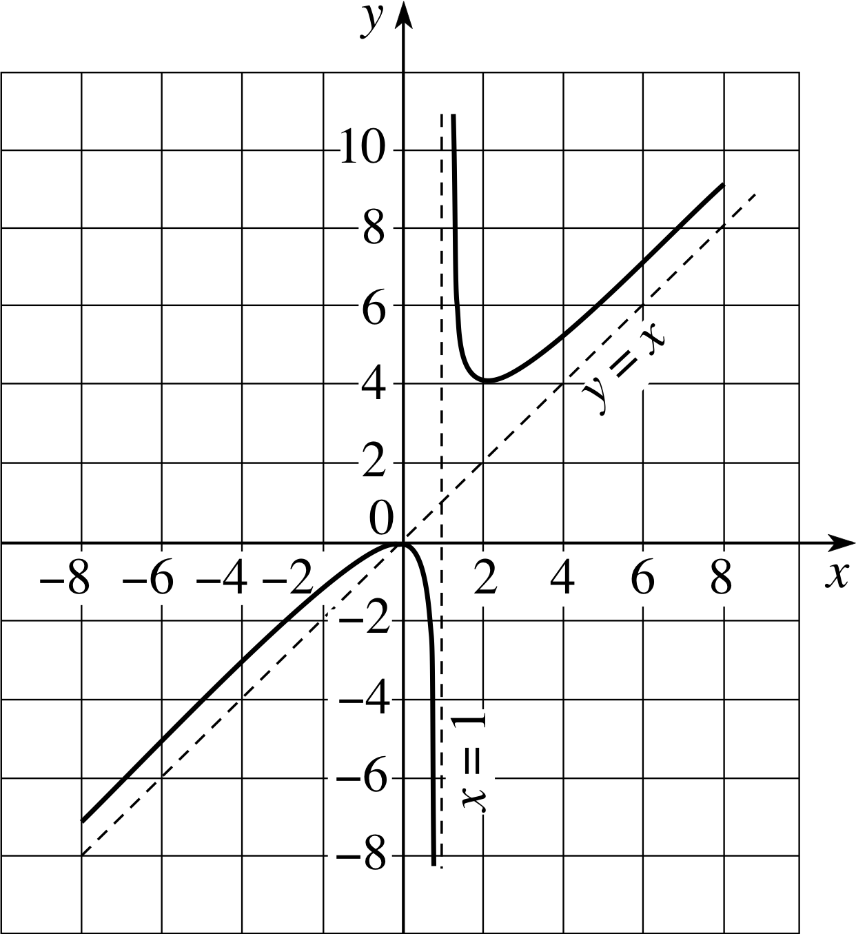
Figure 19 Sketch graph of $f(x) = \dfrac{x^2}{x-1}$.
Applying the previous techniques we can examine the function
$f(x) = \dfrac{x^2}{x-1}$
We first notice that the function is undefined for x = 1; then we see that it has a double root at x = 0 (so the graph touches the x–axis at x = 0). For values of x a little less than 1 the function is very large and negative, while for values of x a little more than 1 the function is very large and positive.
For values of | x | ≫ 1 we see that $f(x) = \dfrac{x^2}{x-1} \approx x$ (because x − 1 is ‘roughly the same size as x when | x | ≫ 1’), and so y = x is an asymptote.
Notice that all of the above information was obtained without the use of calculus, but if we need more detail then we can differentiate to obtain (after some manipulation) $f'(x) = \dfrac{x(x-2)}{(x-1)^2}$. So we can see from this that there are stationary points at x = 0 (confirming what we already suspected) and at x = 2.
We must now choose to use either the first or second derivative tests. In this case it is not too difficult to show that $f''(x) = \dfrac{2}{(x-1)^3}$ so we use the second derivative test. We have f ′′ (0) = −2 < 0, so that there is a local maximum at x = 0, and f ′′ (2) = 2 > 0 so that there is a local minimum at x = 2. There are no points of inflection since the second derivative is never zero. i Combining all the information we obtain the sketch graph shown in Figure 19.
8 Concavity
In some circumstances you may find that the concavity provides useful extra information about the curve; however this is not usually the case.
4.3 Examples
In this subsection we sketch the graphs of three functions. In any one example we need some, but not necessarily all, of the techniques outlined in the previous subsection.
Remember that you may not need to obtain all the information that we derive in these examples. The general principle is that you should obtain enough information to produce a sketch that is sufficient to your needs.
Example 1
Sketch the graph of f (x) = (x − 1)2(x − 2).
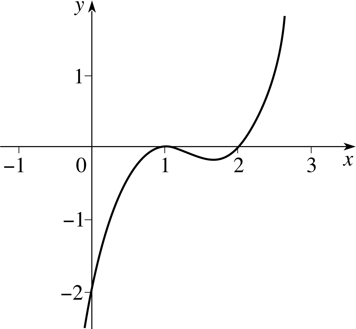
Figure 20 A sketched graph of the function f (x) = (x − 1)2(x − 2).
Solution
(a) We notice that y = f (x) = 0 when x = 1 (a double root) or x = 2 so we have found two intercepts on the x–axis. Also f (0) = −2 gives us the intercept on the y–axis.
(b) If x ≫ 1 then (x − 1)2 ≈ x2 and x − 2 ≈ x so that f (x) ≈ x3, and so we see that the graph approaches y = x3 when | x | ≫ 1.
(c) Differentiating the function we have f ′ (x) = 3x2 − 8x + 5 = (3x − 5)(x − 1) and so there are stationary points at x = 1 (where y = 0) and at x = 5/3 (where y = −4/27).
(d) Differentiating again we have f ′′ (x) = 6x − 8, and since f ′′ (1) = −2 < 0 there is a local maximum at x = 1, while f ′′ (5/3) = 2 > 0 so there is a local minimum at x = 5/3. The graph is therefore concave upwards if 6x − 8 is positive, i.e. x > 4/3, and concave downwards if 6x − 8 is negative, i.e. x < 4/3.
We can now complete the sketch (see Figure 20).
Example 2
Sketch the graph of $g(x) = \dfrac{x}{1+x^2}$.
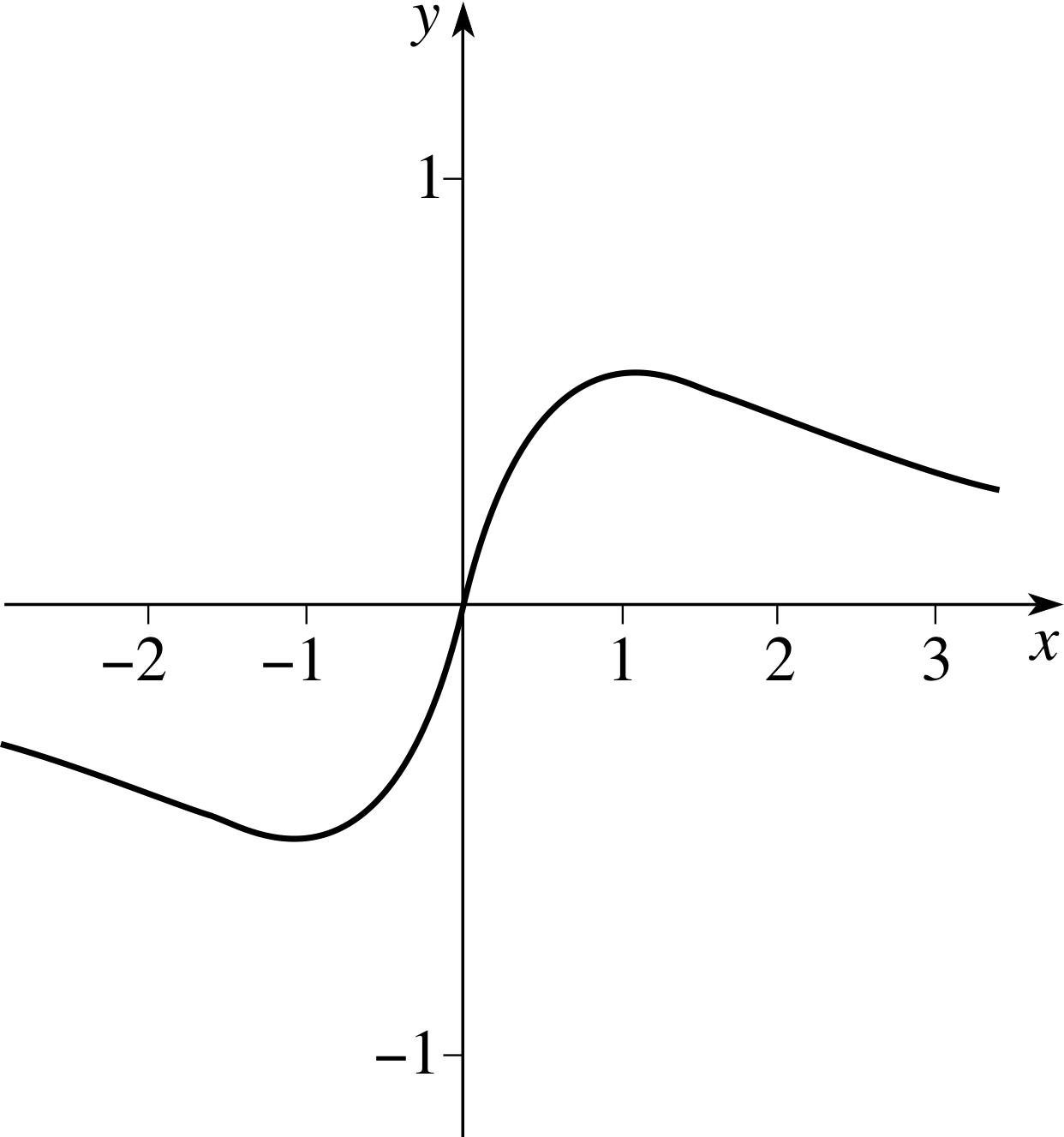
Figure 21 A sketched graph of $g(x) = \dfrac{x}{1+x^2}$
Solution
(a) We first notice that g (0) = 0 and this is the only intercept on the x–axis and on the y–axis. If x ≫ 1 then 1 + x2 ≈ x2 so that g (x) ≈ 1/x and the graph approaches y = 1/x. If x ≪ 1 then x2 is small compared to 1 and x, so that g (x) ≈ x, and therefore the tangent at x = 0 is y = x.
(b) Since g (−x) = −g (x) the function is odd (despite mixing odd and even powers of x); moreover g (x) > 0 when x > 0, and g (x) < 0 when x < 0. It follows that no part of the graph appears in the region where y > 0 when x < 0, nor in the region where y < 0 when x > 0.
(c) Differentiating we see that $g'(x) = \dfrac{(1 - x^2)}{\left(1+x^2\right)^2}$ and so there are stationary points (when 1 − x2 = 0) at x = 1 (where y = 1/2) and at x = −1 (where y = −1/2).
(d) In this case we may choose to use the first derivative test, and we see that g ′ (x) < 0 if x > 1 or x < −1 and g ′ (x) > 0 if −1 < x < 1. The function is therefore decreasing for x < −1, increasing for −1 < x < 1 and decreasing for x > 1. It follows that there is a local minimum at x = −1 and a local maximum at x = 1.
(e) At x = 0 we have g ′ (x) = 1, confirming that the tangent is y = x at the origin.
(f) If necessary we could find the second derivative $g''(x) = \dfrac{2x(x^2 - 3)}{\left(x^2+1\right)^3}$ and the fact that g ′′ (−1) = 0.5 > 0 while g ′′ (1) = −0.5 to confirm that x = −1 is a local minimum and x = 1 is a local maximum, from the second derivative test. The second derivative changes sign at x = 0 and at $x = \pm\sqrt{3\os}$ so that these are points of inflection.
All of this information can now be used to produce a sketch of the graph as in Figure 21.
Example 3
Sketch the graph of $h(x) = \dfrac{x}{{\rm e}^x}$.
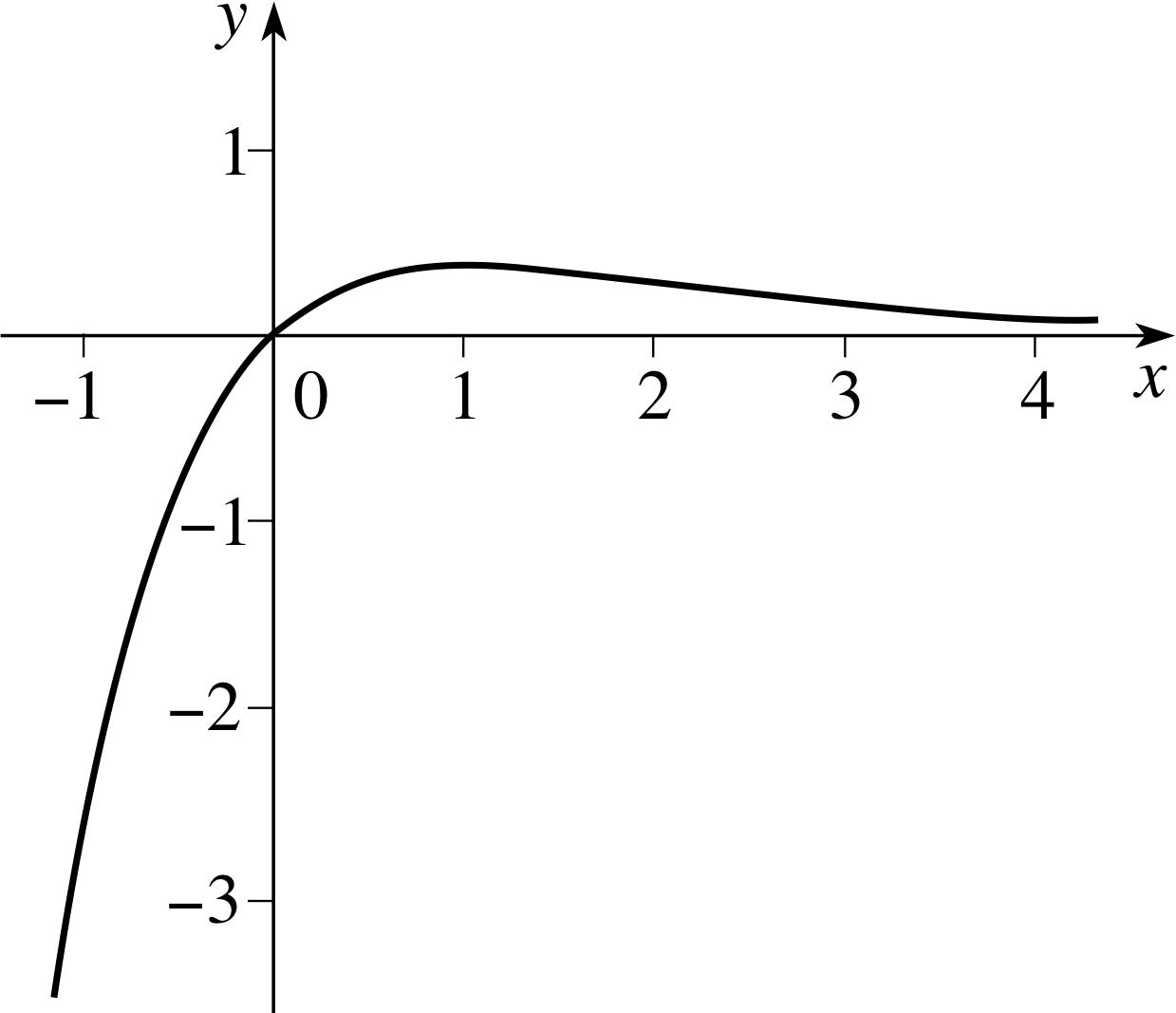
Figure 22 A sketched graph of $h(x) = \dfrac{x}{{\rm e}^x}$.
Solution
(a) We notice that h (x) = 0 at x = 0 (and this is the only intercept on the x–axis and on the y–axis).
(b) For x ≫ 1 the value of ex is considerably larger than x so that h (x) ≈ 0. On the other hand, for x ≪ 1, ex is very small and positive so that h (x) is then large and negative. i
(c) Differentiating we see that $h'(x) = \dfrac{1-x}{{\rm e}^x}$ so that there is a stationary point at x = 1.
(d) Differentiating again we see that $h''(x) = \dfrac{x-2}{{\rm e}^x}$ and, since
h ′′ (1) = −1/e < 0, it follows that there is a local maximum at x = 1. The second derivative changes sign at x = 2 so that this is a point of inflection. See Figure 22.
Question T10
Sketch the graphs of the following functions:
(a) $f(x) = x - \dfrac1x$, (b) f (x) = x4 − 4x3 + 10, (c) f (x) = x4 − x2.
Answer T10
(a) This is an odd function. The graph intercepts the x–axis
when x = ±1. f (x) ≈ −1/x when | x | is small and f (x) ≈ x when | x | is large. Also $f'(x) = 1 + \dfrac{1}{x^2} \gt 0$.
Hence there are no stationary points, and, since f ′ (x) > 0 for all x (except x = 0), f (x) is increasing if x < 0 and also increasing if x > 0.
The graph is sketched in Figure 25.
(b) f ′ (x) = 4x3 − 12x2 = 4x2(x − 3). By the first derivative test, x = 0 is a point of inflection, x = 3 is a local minimum. f (0) = 10, f (3) = −17. f (x) = 0 for x ≈ 1.6 and 3.8. For large x, f (x) ≈ x2.
The graph is sketched in Figure 26.
(c) f (x) is an even function and f (−1) = f (0) = f (1) = 0.
f ′ (x) = 2x (2x2 − 1), f ′′ (x) 12x2 − 2, f ′ (x) = 0 at x = 0, $\pm 1/\sqrt{2\os}$.
Using the second derivative test we find that x = 0 is a local maximum, $x = \pm 1/\sqrt{2\os}$ are local minima, and that there are points of inflection at $x = \pm 1/\sqrt{6\os}$ (since f ′′ (x) changes sign at these points).
The graph is sketched in Figure 27.
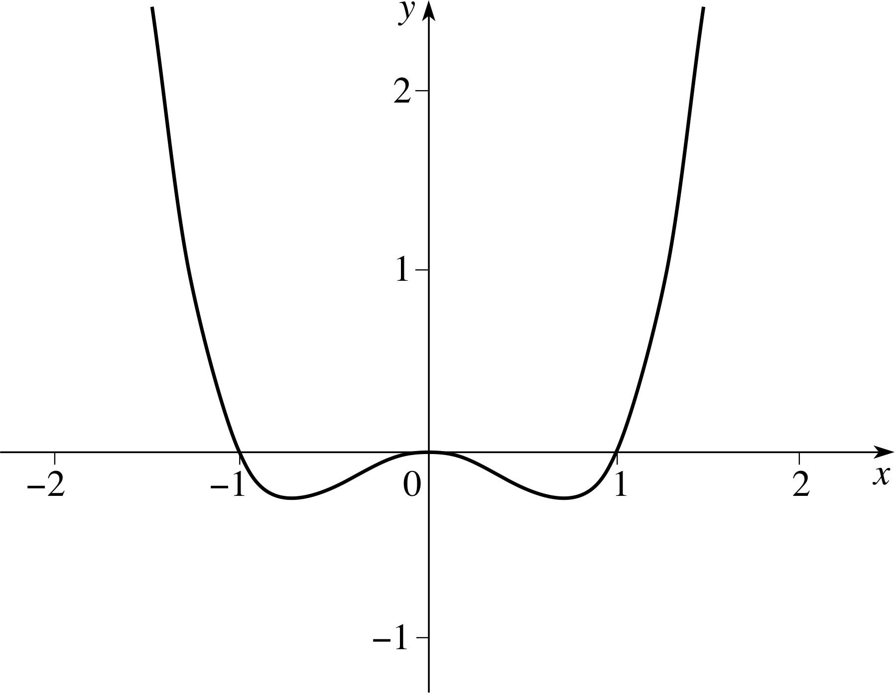
Figure 27 See Answer T10(c).
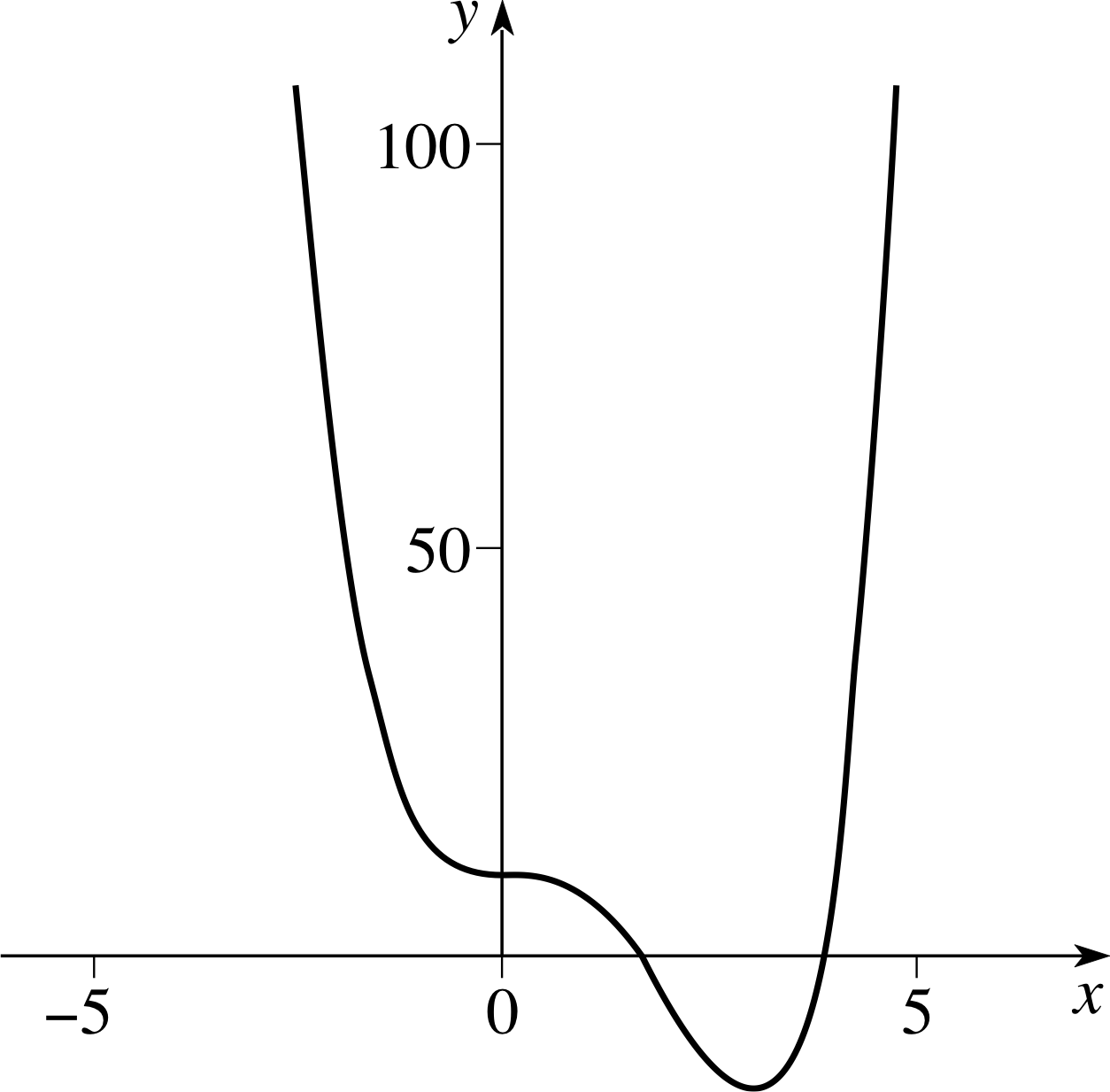
Figure 26 See Answer T10(b).
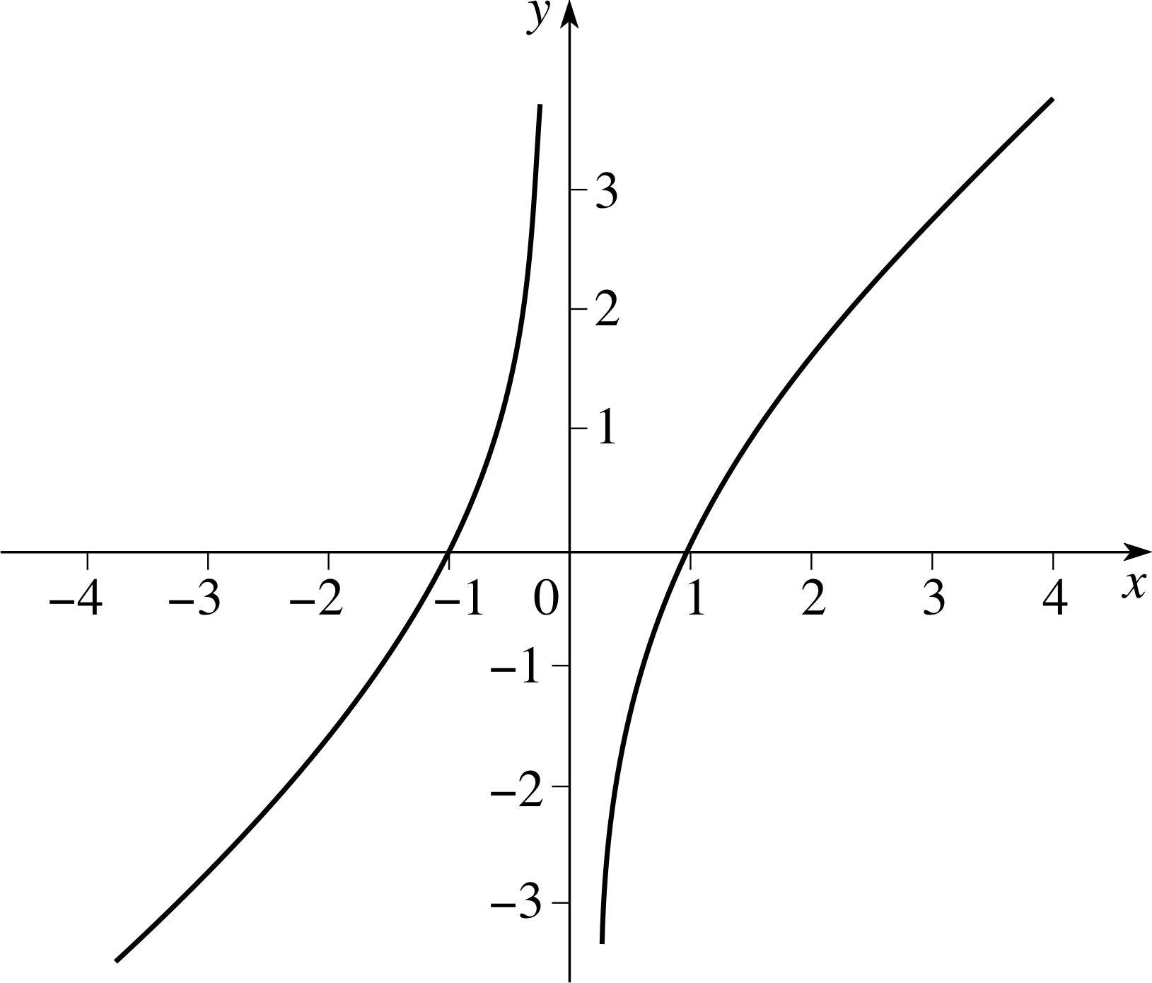
Figure 25 See Answer T10(a).
5 Closing items
5.1 Module summary
- 1
-
In order to discover the global maximum (or minimum) of a given function in an interval a ≤ x ≤ b:
(a) First ensure that the function is defined at every point of the interval. If this is not the case there may be no global maximum or minimum.
(b) Evaluate the function at any points where the derivative is undefined.
(c) Evaluate the function at the end points of the interval.
(d) Evaluate the function at the stationary points (i.e. points where the derivative of the function is zero).
The global maximum is the greatest, and the global minimum the least, of these values.
- 2
-
To find the local maxima and minima of a given function, f (x) say:
(a) Find the stationary points (the points at which f ′ (x) = 0).
(b) If it is easy to find the second derivative, evaluate f ′′ (x) at the stationary points. Then:
(i) A positive second derivative indicates a local minimum.
(ii) A negative second derivative indicates a local maximum.
(iii) If the second derivative is zero at the stationary point one must investigate further:
If f ′′ (x) changes sign at the stationary point then the point is a point of inflection (with horizontal tangent).
If f ′′ (x) does not change sign at the stationary point then either: f ′′ (x) > 0 near the point, which means that the graph is concave upwards, and there is a local minimum; or, f ′′ (x) < 0 near the point, which means that the graph is concave downwards, and there is a local maximum.
(c) If it is not easy to calculate f ′′ (x), examine the behaviour of f ′ (x) near the stationary point.
(i) If f ′ (x) changes sign at the stationary point then this point is a turning point, and must therefore be a local maximum or a local minimum. If f ′ (x) changes from negative to positive there is a local minimum. If f ′ (x) changes from positive to negative there is a local maximum.
(ii) If f ′ (x) does not change sign at the stationary point then this point is a point of inflection.
(d) If the first and second derivative test are too difficult to apply, simply investigate the value of f (x) at values of x that are close to the stationary point.
- 3
-
In order to Section 4sketch the graph of a function, the following points may be considered:
(a) The symmetry of the function. Is it even (f (−x) = f (x)) or odd (f (−x) = −f (x)) ?
(b) Intervals or points where the function is undefined.
(c) Points at which the graph crosses the axes. Do the intersections on the x–axis correspond to multiple roots?
(d) Behaviour of the graph near points at which the function is undefined. Are there any asymptotes?
(e) Behaviour of the graph when | x | ≫ 1. Does the graph approach some simple curve?
(f) Behaviour of the graph where | x | ≪ 1. What is the tangent at the origin?
(g) Points at which the function is stationary. Are these turning points or points of inflection (with a horizontal tangent)? Where is the function increasing and where is it decreasing?
(h) Where is the graph concave upwards and where is it concave downwards?
5.2 Achievements
Having completed this module, you should be able to:
- A1
-
Define the terms that are emboldened and flagged in the margins of the module.
- A2
-
Define increasing and decreasing functions.
- A3
-
Define global and local extrema.
- A4
-
Locate the stationary points of a function.
- A5
-
Define a point of inflection.
- A6
-
Identify the nature of the stationary points of a function using both first and second derivatives.
- A7
-
Distinguish between odd and even functions, and recognize the graphs of such functions.
- A8
-
Sketch the graph of a function from its formula showing its main features.
Study comment You may now wish to take the following Exit test for this module which tests these Achievements. If you prefer to study the module further before taking this test then return to the topModule contents to review some of the topics.
5.3 Exit test
Study comment Having completed this module, you should be able to answer the following questions, each of which tests one or more of the Achievements.
Question E1
(A3 and A4) Find the stationary points on the graph of y = x2 + x and on the graph of y = x2 − x.
Explain why the function f (x) = x2 + | x | has no stationary points, and find its global maximum value in the interval −1 ≤ x ≤ 1.
Answer E1
If y = x2 + x then dy/dx = 2x + 1 so that there is a stationary point at x = −1/2. If y = x2 −x then dy/dx = 2x − 1 so that there is a stationary point at x = 1/2.
The function f (x) = x2 + | x | can be differentiated everywhere except at x = 0. Thus,
f (x) = x2 + x and f ′ (x) = 2x + 1 if x > 0
f (x) = x2 − x and f ′ (x) = 2x − 1 if x < 0
so that f (x) has no stationary points since its derivative is not zero at any point. To find its global maximum over −1 ≤ x ≤ 1 we need only examine the values of f (x) at the ends of the interval and at x = 0. f (−1) = 2, f (0) = 0, f (1) = 2. We see that the global maximum is 2.
(Reread Subsection 2.3Subsections 2.3 and Subsection 2.62.6 if you had difficulty with this question.)
Question E2
(A2, A3, A4, A5 and A6) Find any local maxima, local minima and points of inflection of the function
f (x) = 6x5 − 10x3
Answer E2
f ′ (x) = 30x4 − 30x2 = 30x2(x2 − 1) and f ′′ (x) = 120x3 − 60x = 60x (2x2 − 1)
There is a local maximum at x = −1, a local minimum at x = 1, and points of inflection at x = 0 and $x = \pm 1/\sqrt{2\os}$. Note that the function is odd, which supports these conclusions.
(Reread Subsection 2.4Subsections 2.4, Subsection 2.52.5, Subsection 3.23.2 and Subsection 3.33.3 if you had difficulty with this question.)
Question E3
(A3, A4 and A6) A closed container is to be constructed in the shape of a circular cylinder of volume 16π (metre)3. What dimensions should it have if the total surface area is to be a minimum? i
Answer E3
Let the radius of the cylinder be r and the height be h.
Then πr2h = 16π (metre)3 so that h = (16 m3)/r2.
The total surface area S is given by
$S = 2\pi r^2+ 2\pi rh = 2\pi r^2+ \dfrac{(32\,{\rm m}^3)\pi r}{r^2} = 2\pi r^2 + \dfrac{(32\,{\rm m}^3)\pi}{r}$
$\dfrac{dS}{dr} = 4\pi r - \dfrac{(32\,{\rm m}^3)\pi}{r^2} = \dfrac{4\pi(r^3-8\,{\rm m}^3)}{r^2}$
which is zero when r = 2 m
$\dfrac{d^2S}{dr^2} = 4\pi + \dfrac{(64\,{\rm m}^3)\pi}{r^3} \gt 0$ if r > 0
Hence r = 2 m gives a local minimum which can be seen to be a global minimum (since S is large when | r | is either very small or very large).
The required dimensions are therefore r = 2 m and h = 4 m.
(Reread Subsection 2.4Subsections 2.4, Subsection 2.52.5, Subsection 3.23.2 and Subsection 3.33.3 if you had difficulty with this question.)
Question E4
(A7 and A8) Sketch the graph of the function
$f(x) = \dfrac{x^2+3}{x+1}$
Answer E4
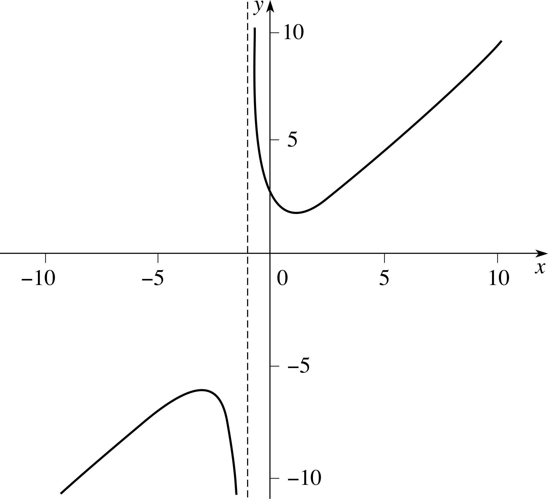
Figure 28 See Answer E4.
The function is neither even nor odd. When x = 0, f (x) = 3. The graph has no intercepts with the x–axis. The function is not defined for x = −1.
If x is a little greater than −1 then f (x) is large and positive. If x is a little less than −1 then f (x) is large and negative.
As | x | → ∞, f (x) ≈ x
$f'(x) = \dfrac{(x + 1)2x - (x^2+ 3)}{(x+1)^2} = \dfrac{x^2+2x-3}{(x+1)^2} = \dfrac{(x + 3)(x-1)}{(x+1)^2}$
f ′ (x) > 0 if x > 1 or x < −3 so f (x) is increasing if x < −3 or x > 1.
f ′ (x) < 0 if −3 < x <−1 and −1 < x < 1, so f (x) is decreasing in the interval −3 < x <−1 and also decreasing in the interval −1 < x < 1.
x = 1 is a local minimum. x = −3 is a local maximum.
The graph of y = x + 1 is sketched in Figure 28.
(Reread Section 4 if you had difficulty with this question.)
Study comment This is the final Exit test question. When you have completed the Exit test go back and try the Subsection 1.2Fast track questions if you have not already done so.
If you have completed both the Fast track questions and the Exit test, then you have finished the module and may leave it here.
Study comment Having seen the Fast track questions you may feel that it would be wiser to follow the normal route through the module and to proceed directly to the following Ready to study? Subsection.
Alternatively, you may still be sufficiently comfortable with the material covered by the module to proceed directly to the Section 5Closing items.