MATH 5.2: Basic integration |
PPLATO @ | |||||
PPLATO / FLAP (Flexible Learning Approach To Physics) |
||||||
|
1 Opening items
1.1 Module introduction
Integration enters into almost every area of physics, and it does so in two quite different ways. On the one hand, the process known as indefinite integration allows us, up to a point, to reverse the effect of differentiation and is therefore of importance wherever differentiation arises, i.e. almost everywhere. On the other hand, the process of definite integration allows us to extend the idea of summation to the addition of continuous distributions. For example, a column of air will have a density that increases continuously from its top to its bottom, yet definite integration allows us to add together the mass of each layer in the column and, in an appropriate limit, evaluate the total mass of the column. Both aspects of integration – reversing differentiation and finding limits of sums – are important in their own right, but they take on increased significance when they are brought together by the fundamental theorem of calculus, since it allows us to use indefinite integrals in the evaluation of many definite integrals.
This module contains three main sections, the first (Section 2) deals with fundamental principles and definitions. It reviews important concepts such as function, variable and graph, introduces indefinite and definite integration, and explains how definite integrals (the limits of sums) can be interpreted in terms of the area under the graph of a function. Along the way it introduces the fundamental theorem of calculus, arguably the most important result in the study of integration.
Section 3 of the module is mainly concerned with the determination of indefinite integrals. It contains two tables of standard indefinite integrals, (the more basic in Subsection 3.1 and the more advanced in Subsection 3.3) and sandwiched between them are various rules for integrating combinations of functions whose individual indefinite integrals are already known. It almost goes without saying that this section, with its emphasis on simple functions, is only scratching the surface of a very large topic; other techniques of integration are dealt with elsewhere in FLAP.
Section 4 concerns definite integrals. It lists the general mathematical properties of definite integrals and looks at the special simplifications that occur in the physically important cases where the functions being integrated are odd, even or periodic. The section concludes with a discussion of improper integrals that may involve integrating over an infinite range of values, or integrating a function which itself becomes infinite at some point in the range of integration.
Study comment Having read the introduction you may feel that you are already familiar with the material covered by this module and that you do not need to study it. If so, try the following Fast track questions. If not, proceed directly to the Subsection 1.3Ready to study? Subsection.
1.2 Fast track questions
Study comment Can you answer the following Fast track questions? If you answer the questions successfully you need only glance through the module before looking at the Subsection 5.1Module summary and the Subsection 5.2Achievements. If you are sure that you can meet each of these achievements, try the Subsection 5.3Exit test. If you have difficulty with only one or two of the questions you should follow the guidance given in the answers and read the relevant parts of the module. However, if you have difficulty with more than two of the Exit questions you are strongly advised to study the whole module.
Question F1
A function f (x) is positive in an interval a ≤ x ≤ b. Explain how the area under the graph of f (x) between x = a and x = b can be represented as a definite integral. What are the magnitudes of the various areas enclosed by the graph of y = x3, the x–axis and the lines x = −2 and x = 1? (Note that this graph crosses the horizontal axis at x = 0).
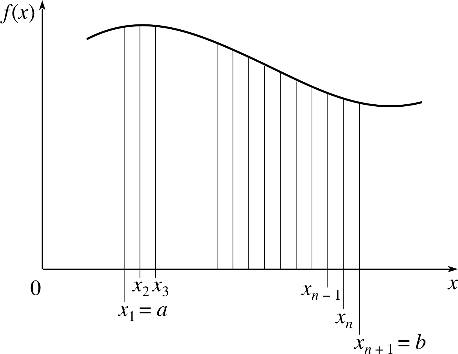
Figure 5 The area under the graph of an arbitrary function may be approximated by a sum of rectangles.
Answer F1
The area under the curve is divided into n thin strips of width ∆xiand height f (xi), as shown in Figure 5. The approximate area of such a strip is f (xi)∆xi, and the total area is $\left(\displaystyle \sum_{i=1}^nf(x_i)\Delta x_i\right)$ where the summation is taken over all strips. As the number of strips increases and the width of each strip decreases, this summation tends to ${\Large\int}_a^bf(x)\,dx$, which is the exact area required.
When the graph crosses the x–axis at a point c where a < c < b, each region where f (x) has a fixed sign must be considered separately.
Thus the magnitudes of the enclosed areas in the case f (x) = x2, where the graph crosses the horizontal axis at x = 0, will be
$A_1 = \left\vert{\Large\int}_{-2}^0x^3\,dx\,\right\vert = \left\vert\left[\dfrac{x^4}{4}\right]_{-2}^0\,\right\vert = \left\vert\,0 - \dfrac{16}{4}\,\right\vert = 4$
and$A_2 = \left\vert{\Large\int}_0^1x^3\,dx\,\right\vert = \left\vert\left[\dfrac{x^4}{4}\right]_0^1\,\right\vert = \dfrac14$
Question F2
Find the following indefinite integrals:
(a) ${\Large\int}(4x^2 + 7x - 5)\,dx$
(b) ${\Large\int}{\rm e}^{-6x}\,dx$
(c) ${\Large\int}\left[3\cos(4x) - 5\sin(4x)\right]\,dx$
(d) ${\Large\int}3\loge (2x)\,dx$
Answer F2
(a) ${\Large\int}(4x^2 + 7x - 5)\,dx = \frac43x^3 + \frac72x^2 - 5x + C$
(b) ${\Large\int}{\rm e}^{-6x}\,dx = -\frac16{\rm e}^{-6x} + C$
(c) ${\Large\int}\left[3\cos(4x) - 5\sin(4x)\right]\,dx = \frac34\sin(4x) + \frac54\cos(4x) + C$
(d) ${\Large\int}3\loge (2x)\,dx = 3x\loge (2x) - 3x + C$
Question F3
Evaluate the following definite integrals (to four decimal places):
(a) ${\Large\int}_{-2}^3(3 - 2x - x^2)\,dx$
(b) ${\Large\int}_{\pi/4}^{\pi/3}\left[6\cos(3x) - 10\cos(2x)\right]\,dx$
(c) ${\Large\int}_1^24\loge x\,dx$
Answer F3
(a) ${\Large\int}_{-2}^3(3 - 2x - x^2)\,dx = \left[3x - x^2 - \dfrac{x^3}{3}\right]_{-2}^3 = (9-9-9) - \left(-6-4+\dfrac83\right) = - \dfrac53 \approx -1.6667$
(b) ${\Large\int}_{\pi/4}^{\pi/3}\left[6\cos(3x) - 10\cos(2x)\right]\,dx = \left[2\sin(3x) - 5\sin(2x)\right]_{\pi/4}^{\pi/3}$
(b) $\phantom{{\Large\int}_{\pi/4}^{\pi/3}\left[6\cos(3x) - 10\cos(2x)\right]\,dx }= \left(0-\dfrac{5\sqrt{3\os}}{2}\right) - \left(2\times\dfrac{1}{\sqrt{2\os}}-5\times 1\right) = \dfrac{-5\sqrt{3\os}}{2} - \sqrt{2\os} + 5 \approx -0.7443$
(c) ${\Large\int}_1^24\loge x\,dx = 4\left[x\loge x - x\right]_1^2 = 4(2\loge 2 - 1) \approx 1.5452$
1.3 Ready to study?
Study comment To study this module you will need to be familiar with the following terms: constant, derivative, differentiation, function, graph, inequality (in particular the symbols <, >, ≤ and ≥ for inequalityless than, inequalitygreater than, inequalityless than or equal to and inequalitygreater than or equal to), limit, magnitude_of_a_vector_or_vector_quantitymagnitude (of a vector, in the sense of the strength of a force), modulus (as in | −3 | = 3) and summation (including the summation symbol, Σ). In addition you will need to be familiar with the properties of the elementary functions, power_mathematicalpowers, root_of_an_equationroots, reciprocals, exponential_functionexponentials, logarithmic_functionlogarithms and trigonometric functions (including the reciprocal functions and inverse trigonometric functions such as sec(x) and arcsec(x)), and it would be helpful if you were familiar with some of the general terminology of functions (domain, codomain, argument, etc.), though this is reviewed in Subsection 2.1. It is assumed that you are reasonably proficient at differentiation and that you know how to differentiate sums and products of the elementary functions as well as being able to use the chain rule to differentiate functions of functions. Implicit differentiation is used in Subsection 3.3 but lack of familiarity with that technique should not prevent you from studying the module. Finally, you will need to have some idea of what it means to take the limit of an expression. If you are uncertain about any of these topics you can review them by referring to the Glossary which will also indicate where in FLAP they are developed. The following questions will allow you to establish whether you need to review some of the topics before embarking on this module.
Note that throughout this module x represents the positive square root of x.
Question R1
For each of the following functions find the derivative f ′ (x) = df /dx:
(a) f (x) = 8x6 + 6x3 − 5x2 − 2, (b) f (x) = 3 sin(x) + 4 cos(x), (c) f (x) = 5 e2x − 2 e−2x, (d) f (x) = 2 logex + 3 loge(2x)
Answer R1
(a) df /dx = 48x2 + 18x2 − 10x
(b) df /dx = 3 cos(x) − 4 sin(x)
(c) df /dx = 10 e2x + 4 e−x
(d) $\dfrac{df}{dx} = \dfrac2x + \dfrac3x$
Question R2
Find dy/dx for each of the following equations:
(a) y = 5 cos(x) + 2x2 − 7x, (b) y = 6 e−3x, (c) y = x2 − 5 logex
Answer R2
(a) $\dfrac{dy}{dx} = 5\sin(x) + 4x - 7$
(b) $\dfrac{dy}{dx} = -18{\rm e}^{-3x}$
(c) $\dfrac{dy}{dx} = 2x - \dfrac5x$
Consult derivative in the Glossary for further information.
Question R3
Evaluate the following
(a) $\displaystyle \lim_{x\rightarrow 1}{(2-x)}$ (i.e. the limit as x tends to 1 of (2 − x))
(b) $\displaystyle \sum_{i=1}^32i$ (i.e. the sum from i = 1 to i = 3 of 2i)
(c) arcsin(−1) (i.e. the inverse sine of −1)
Answer R3
(a) $\displaystyle \lim_{x\rightarrow 1}(2 - x) = 1$
(b) $\displaystyle \sum_{i=1}^32i = 2 + 4 + 6 = 12$
(c) arcsin(−1) = −π/2 = nπ/2, where n = −3, −2, −1, 2, 3, 5, ...
Consult limit, summation and inverse trigonometric functions in the Glossary for further information.
2 Principles of integration
2.1 Functions, variables and graphs
Study comment An understanding of functions is crucial to an understanding of integration, and it is vital that the notation and terminology used to describe functions should be clear and unambiguous. For that reason, this subsection reviews the definitions of terms such as function and variable even though it is assumed that you have met these ideas before. If you are completely unfamiliar with these concepts you can locate a more introductory treatment by consulting the entry on functions in the Glossary.
The temperature of a cooling cup of coffee varies with time; the frequency of vibration of a stretched string is determined by its length. We can describe these relationships by saying that the coffee’s temperature is a function of time, or that the string’s frequency is a function of its length.
Mathematically, a function f is a rule that assigns a single value f (x) i in a set called the codomain to each value x in a set called the domain.
Functions are usually defined by formulae, for example f (x) = x2, and in such cases we assume, unless we are told otherwise, that the domain is the largest set of real values i for which the formula makes sense.
In the case of f (x) = x2 the domain of the function is the set of all real numbers. The function $g(x) = \dfrac{1}{1-x}$ is not defined when x = 1, since 1/0 has no meaning, and so we take the set of all real numbers x with x ≠ 1 as its domain.
The function
f (x) = 1 + x + x2(1a)
is another example of a function that is defined for all values of x. One may think of the function as a sort of machine with x as the input and 1 + x + x2 as the output. The input x is known as the independent variable and, if we write y = f (x), the output y is known as the dependent variable, since the function f (x) determines the way in which y depends on x.
The same function f could equally well be defined using some other symbol, such as t, to represent the independent variable:
f (t) = 1 + t + t2(1b)
This freedom to relabel the independent variable is often of great use, though it is vital that such changes are made consistently throughout an equation.
We may evaluate the function in Equation 1, whether we call it f (x) or f (t), for any value of the independent variable; for example, if we choose to use x to denote the independent variable, and set x = 1, we have
f (1) = 1 + 1 + 12 = 3
Similarly, if x = π
f (π) = 1 + π + π2
and, if x = 2a
f (2a) = 1 + 2a + (2a)2 = 1 + 2a + 4a2
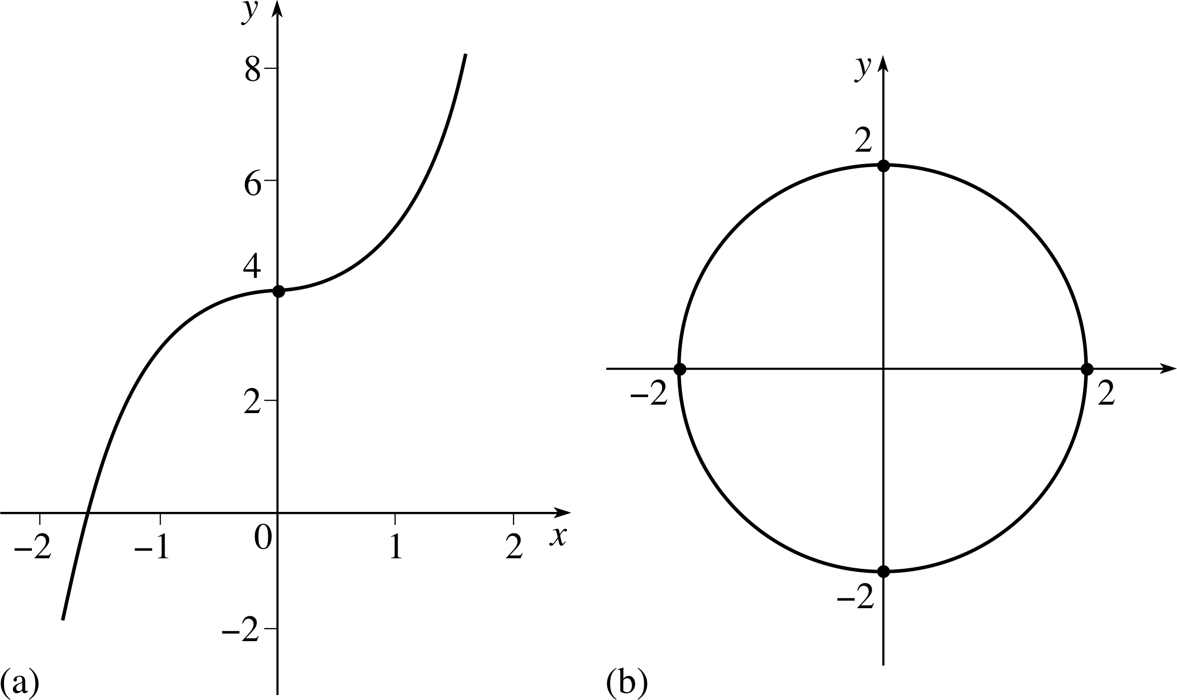
Figure 1 (a) Graph of y = x3 + 4. (b) The circle x2 + y2 = 4. (Part (b) is an example of a relationship that does not fit the strict definition of a function.)
When we write expressions such as f (π) or f (2a) whatever appears within the brackets is called the argument of the function. The value of f (x) is determined by the value of its argument, irrespective of what we call the argument.
We can often learn a great deal about a function f (x) by considering its graph which is a plot of the points (x, f (x)).
Figure 1a depicts part of the graph of the function f (x) = x3 + 4; for the purposes of drawing the graph we have written the relationship as y = x3 + 4.
In Figure 1b we have drawn the graph of the relationship
x2 + y2 = 4
Strictly speaking, this relationship is not a function because for each value of x in the interval −2 < x < 2 there are two values of y; this is not possible for a function.
Question T1
Which of the following expressions define y as a function of x?
(a) y = (x + 2)2, (b) $y = \sqrt{x\os}$ (where $\sqrt{x\os}$ is the positive square root of x), (c) y2 = x, (d) y = 2, (e) y2 = 2
Answer T1
(a) This is a function, every value of x gives rise to a unique value for y.
(b) This is a function because we are taking $\sqrt{x\os}$ to be the positive square root of x in this module. (Note that if we were following the common convention of allowing $\sqrt{x\os}$ to denote either of the square roots of x, so that $\sqrt{4\os}$ = ±2, then x would not have defined a function.)
(c) This definitely does not define y as a function of x. For each positive value of x there are two possible values of y.
(d) Perhaps it is a surprise, but this does define y as a function of x, it is a constant function, f (x) = 2. (e) In this case y = ±2, so y is not uniquely defined and so cannot be a function of x.
2.2 Indefinite integrals: reversing differentiation
If the height x (in metres) of an object above ground level at time t (in seconds) is given by the function
x (t) = (400 m) − ½ gt2(2)
where g = 9.81 m s−2, then it is a straightforward matter of differentiating the equation to obtain an expression for the velocity vx of the object in the x–direction, as a function of time.
$v_x(t) = \dfrac{dx}{dt} = -gt$(3) i
However, the reverse process is not possible, i.e. given vx = −gt we cannot find a formula for the height of the object above ground level. At least, not quite! Any one of the formulae for x below would give the same formula for vx even though none of them agrees with Equation 2,
x (t) = (3 m) − ½ gt2(4a)
x (t) = − ½ gt2(4b)
x (t) = (−5 m) − ½ gt2(4c)
Indeed, on the basis of Equation 3, the most we can really say about x (t) is that it is of the form
x (t) = C − ½ gt2(5)
where C may be any constant. In order to discover that C should be 400 m in this case we need an additional piece of information, such as the position of the object at a particular time. In the absence of appropriate additional information we just have to accept that the value of the arbitrary constant C cannot be determined.
So, we can reverse the process of differentiation, but only up to a point. Since the derivative of any constant is zero we must accept that when we try to work back from the derivative to the function our answer is bound to include an arbitrary additive constant, the value of which cannot be determined without the aid of additional information.
Now, despite its ambiguities, the process of reversing differentiation in the sense we have just been discussing is of great importance in physics and mathematics. It is sometimes referred to as inverse differentiation or antidifferentiation, which captures its spirit, but is more often called indefinite integration. It has its own notation and terminology, which, like the d/dx notation of differentiation, was introduced by Gottfried Wilhelm Leibniz (1646–1716).
If f (x) is a given function and F (x) is any function such that
$\dfrac{dF}{dx} = f(x)$ then we write $F(x) = \int f(x)\,dx$
and we call F (x) an indefinite integral of f (x). i
So, we can say that
${\Large\int}3x^3\,dx = 3x^4 + C$ since $\dfrac{d}{dx}\left(3x^4 + C\right) = 3x^3$(6)
and we might similarly write
${\Large\int}gt\,dt = \dfrac12gt^2 + C$ since $\dfrac{d}{dt}\left(\dfrac12gt^2 + C\right) = gt$(7)
or${\Large\int}4y^2\,dy = \dfrac43y^3 + C$ since $\dfrac{d}{dx}\left(\dfrac43y^3 + C\right) = 4y^2$(8)
Note that in each case we have found the indefinite integral ‘by inspection’, based on our knowledge of derivatives, and we have taken care to include an arbitrary constant which we have called C. The fact that we have used the same symbol in each case doesn’t mean that these constants are necessarily the same, it is simply conventional when writing down an indefinite integral to indicate the presence of the constant by means of a letter and C is the most obvious choice. Also note that we have deliberately chosen to use a different independent variable in each case, to emphasize that there is nothing ‘special’ about x.
When discussing indefinite integrals such as Equations 6, 7 or 8, the symbol ∫ is called the integral sign, the function being integrated (e.g. 3x3 in Equation 6, or gt in Equation 7) is called the integrand, and the symbol that terminates the integral (such as the dx in Equation 6) is called the integration element. The integration element has the important job of telling us the integration variable with respect to which the integration is to be performed. Without the dt in Equation 7 you might have forgotten that g was a constant, mistaken it for a variable, and integrated with respect to g. The arbitrary constant (C) that appears each time we determine an indefinite integral is called the constant of integration. Thus, we can read the left–hand side of Equation 8 as ‘the (indefinite) integral of 4y2, with respect to y’.
✦ How would you write using the correct symbol notation ‘the indefinite integral of x3 with respect to x is $\dfrac14x^4$ plus some arbitrary constant’?
✧ $\int{x^3}dx = \frac14x^4 + C$
✦ Which of the following are indefinite integrals of f (x) = 3x2?
(a) x3, (b) 2x3, (c) x3 − 4, (d) x3 + 0.5, (e) x3 + x
✧ (a), (c) and (d)
You will notice that the correct answers to this last question, x3, x3 − 4 and x3 + 0.5 (which are all indefinite integrals of 3x2), only differ from one another by a constant. This is to be expected from our general discussion of indefinite integrals, but it still deserves emphasis since the arbitrary constant C is often overlooked, and its omission is the cause of many errors.
If F1(x) and F2(x) are both indefinite integrals of the same function f (x), then there exists a constant K such that
F1(x) = F2(x) + K i
An obvious consequence of this is that if F (x) is an indefinite integral of f (x) then F (x) + C, where C is any constant, is also an indefinite integral of f (x).
Question T2
Show that if F (x) is an indefinite integral of f (x) then aF (x) is an indefinite integral of the function af (x) where a is a constant. Further, if G (x) is an indefinite integral of another function g (x) show that F (x) + G (x) is an indefinite integral of the function f (x) + g (x). Write down an indefinite integral of the function af (x) + bg (x) where b is a constant.
Answer T2
Since F (x) is an indefinite integral of f (x) we know that
$\dfrac{dF}{dx} = f(x)$
Thus,$\dfrac{d}{dx}[aF(x)] = a\dfrac{d}{dx}[F(x)] = af(x)$
Hence aF (x) is an indefinite integral of af (x).
$\dfrac{d}{dx}[F(x)+G(x)] = \dfrac{d}{dx}[F(x)] + \dfrac{d}{dx}[G(x)] = f(x) + g(x)$
Hence F (x) + G (x) is an indefinite integral of f (x) + g (x).
An indefinite integral of af (x) + bg (x) is aF (x) + bG (x).
Comment Note that we can also add an arbitrary constant to any of these indefinite integrals to obtain another indefinite integral.
Question T3
Find the following indefinite integrals:
(a) $\int 3\,dx$, (b) $\int x^5\,dx$, (c) $\int 5x^{1/4}\,dx$
Answer T3
(a) 3x + C, (b) $\dfrac{x^6}{6} + C$, (c) 4x5/4 + C.
Comment The indefinite integral xp where the power p ≠ −1 is:
$\dfrac{x^{p+1}}{p+1} + C$
Question T4
Verify the following results by differentiation:
(a) $\displaystyle \int\dfrac{1}{\sqrt{2x+2\os}}\,dx = \sqrt{2x+2\os} + C$
(b) ${\Large\int}(x^2 - 2x)^8(x-1)\,dx = \frac{1}{18}(x^2-2x)^9 + C$
(c) $\displaystyle \int\dfrac{\cos x}{(2+\sin x)^2}\,dx = -\dfrac{1}{2+\sin x} + C $
Answer T4
(a) $\dfrac{d}{dx}\left(\sqrt{2x+2\os} + C\right) = \dfrac{d}{dx}\left[(2x+2)^{1/2} + C\right] = \dfrac{1}{\sqrt{2x+2\os}}$
(b) $\dfrac{d}{dx}\left[\dfrac{1}{18}(x^2-2x)^9 + C\right] = \dfrac{1}{18}\times 9(x^2 - 2x)^8(2x-2) = (x^2 - 2x)^8(x-1)$
(c) $\dfrac{d}{dx}\left(-\dfrac{1}{2+\sin x} + C\right) = \dfrac{d}{dx}\left[-(2+\sin x)^{-1} + C\right] = (2+\sin x)^{-2}(\cos x) = \dfrac{\cos x}{(2+\sin x)^2}$
2.3 Definite integrals: the limit of a sum
Up to now we have been concerned with indefinite integration, the reverse process to differentiation; however, there is another kind of integration, definite integration, that is closely related to summation.
Formulating definite integrals i
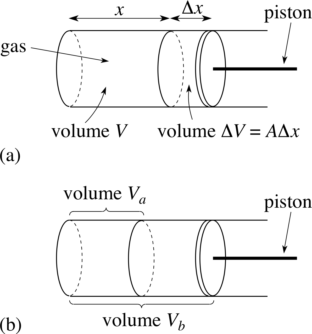
Figure 2 (a) Expansion of a gas by a small amount ∆V = A∆x. (b) A more substantial expansion from an initial value Va to a final volume Vb.
To see how this second kind of integration arises let us consider the physical problem of calculating the work done by an expanding gas. For the sake of simplicity, let us suppose that the gas is confined in a cylindrical vessel (Figure 2a) of cross–sectional area A, by a piston which is free to move in the x–direction. When the position coordinate of the piston is x (measured to the right from the left–hand end of the cylinder), the volume of the gas will be V = xA and we may denote the pressure in the gas by P (V). For a fixed mass of gas at a fixed temperature, this pressure will decrease as V increases.
Whatever its value, the pressure will exert a force in the x–direction on the piston and for a given value of V that force will be
Fx(V) = A × P (V)
If the gas causes the piston to move to the right through a small distance ∆x then the gas will have done a small amount of work ∆W. If the force Fx remained constant throughout this small expansion we could say
∆W = Fx(V) × ∆x
However, Fx will not remain constant throughout the expansion, it will decrease as x increases and the pressure falls. Nonetheless, if we make ∆x very small then the pressure will change very little during the expansion and we can use the approximation
∆W ≈ Fx(V) × ∆x ≈ A × P (V) × ∆x i
As a result of this expansion the volume of the gas will have increased by a small amount ∆V which will be equal to A∆x, so we may rewrite the last result
∆W ≈ Fx(V) × ∆x ≈ A × P (V) × ∆x
as
∆W ≈ P (V)∆V(9)
Now, if we want to calculate the work done by the gas when it increases its volume from an initial value Va to a final volume Vb (Figure 2b), we can do so, at least approximately, by dividing the expansion into many small steps and using Equation 9 to find the work done in each step. To do this we introduce n + 1 values of V such that
Va = V1 < V2 < V3 < ... Vn−1 < Vn < Vn+1 = Vb, i
and we let
∆Vi = Vi+1 − Vi
where i can be any whole number in the range 1 ≤ i ≤ n.
We can then say that the work done by the gas when its volume increases from Vi to Vi + 1 is approximately P (Vi)∆Vi and the total work W done during the expansion is approximately
$\displaystyle P(V_1)\Delta V_1 + P(V_2)\Delta V_2 + P(V_3)\Delta V_3 + \dots + P(V_n\Delta V_n = \sum_{i=1}^nP(V_i )\Delta V_i$(10)
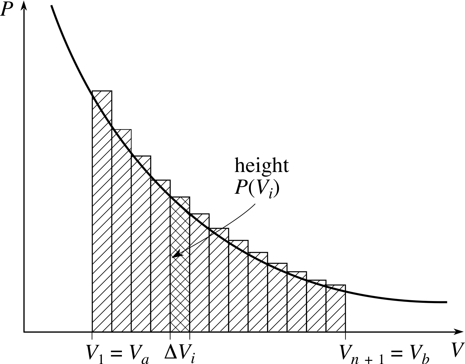
Figure 3 A visualization of Equation 10.
Remember, this is only an approximation to the amount of P work actually done because it erroneously assumes that the pressure is constant throughout each step. (This is indicated graphically in Figure 3, which provides a visualization of Equation 10).
The curve shows the pressure P as a function of the volume V. The work done in any small part of the expansion, from Vi to Vi+1 is approximately represented by the area of the corresponding rectangular strip, P (Vi)∆Vi. The total amount of work done in expanding from Va to Vb is approximately represented by the sum of the areas of the rectangles. Note that as the number of rectangles increases and they become narrower, their total area approaches the area under the graph between Va and Vb; this point is explored in the next subsection.
However, it is an approximation that will become increasingly accurate if we increase the number of steps and let the size ∆Vi of each step become smaller and smaller. Thus, if we take the limit of the above sum as ∆V, the width of the widest step, tends to zero, we have the exact result
$\displaystyle W = \lim_{\Delta V\rightarrow 0}{\left[\sum_{i=1}^nP(V_i)\Delta V_i\right]}$(11)
A limit of a sum of the kind given in Equation 11 is clearly very important (it has real physical significance) but it is also very cumbersome, so such limits of sums are given a special symbol and a special name. They are called definite integrals and the one we have been considering – the definite integral of P (V) with respect to V, from Va to Vb – is denoted by
$\displaystyle W = \int_{V_a}^{V_b}P(V)\,dV$(12) i
As you can see the notation used to denote definite integrals is very similar to that used for indefinite integrals; there is an integral sign, an integrand (P (V) in this case) and an integration element. The only obvious difference is the inclusion of lower_limit_of_integrationlower and upper_limit_of_integrationupper limits of integration, Va and Vb respectively, in the definite integral.
There are good reasons for this similarity, as you will soon see, but you shouldn’t be deceived by it, definite and indefinite integrals are radically different, the indefinite integral of a function is another function, the definite integral of a function between given limits is a value (so many joules in the case of Equation 12) not a function.
Before going on to consider the evaluation of limits of sums, whether we write them as in Equation 11 or use the definite integral notation of Equation 12, it is worth pausing to stress the generality of this concept and its independence of any specific physical context.
This is done as follows:
Given a function f (x) and two values x = a, and x = b, the definite integral of f (x) with respect to x, from a to b is defined by
$\displaystyle \int_a^bf(x)\,dx = \lim_{\Delta x\rightarrow 0}{\left(\sum_{i=1}^nf(x_i)\Delta x_i\right)}$
wherex1 < x2 < x3 < ... xn−1 < xn < xn+1, and ∆xi = xi+1− xi, with x1 = a and xn+1 = b, and ∆x is the largest of the ∆xi.
Evaluating definite integrals
The task of evaluating a limit of a sum may seem a daunting one, and indeed, it can be. However, there are many cases in which the evaluation is really rather straightforward, thanks to the existence of a deep link between definite integrals and indefinite integrals. This link i is embodied in what is arguably the most important result of elementary calculus, the so–called fundamental theorem of calculus:
Fundamental theorem of calculus
If F (x) is any indefinite integral of f (x), so that ${\large\int}f(x)\,dx = F(x)$, then
${\Large\int}_a^bf(x)\,dx = F(b) - F(a)$(13) i
So, if asked to find the definite integral of a given function between given limits, it is easy to do so provided you know, or can work out, an indefinite integral of the given function. Once you have that vital piece of information you only have to evaluate the indefinite integral at the upper and lower limits and then take the difference.
Example 1
Use the fundamental theorem of calculus to evaluate the definite integral ${\Large\int}_1^43x^2\,dx$.
Solution
In this case the integrand of the definite integral is 3x2, and an indefinite integral of this is
$F(x) = {\large\int}3x^2\,dx = x_3 + C$
Consequently, ${\Large\int}_1^43x^2\,dx = F(4) - F(1)$
i.e.${\Large\int}_1^43x^2\,dx = (4^3 + C) - (1^3 + C)$
so${\Large\int}_1^43x^2\,dx = 63$
There are several points to note about this example:
- 1
-
The definite integral is a constant value (63), as expected, not a function of x. This means that the x which appears in the definite integral could have been replaced by any other symbol without affecting the answer. Hence we can be sure that
${\Large\int}_1^43x^2\,dx = {\Large\int}_1^43X^2\,dX = {\Large\int}_1^43{\xi}^2\,d{\xi}$
They are all alternative ways of writing the number 63. A variable that can be replaced in this way without altering the value of an expression is called a dummy variable. In a definite integral the integration variable is always a dummy variable.
- 2
-
The arbitrary constant C that we included in the indefinite integral played no role in the final answer. i This will always be the case and is fully consistent with the fact that the wording of the fundamental theorem allows us to use any indefinite integral of the integrand when evaluating a definite integral. For this reason, when using the fundamental theorem it is conventional to choose the simplest indefinite integral, i.e. that in which C = 0.
- 3
-
Expressions such as F (b) − F (a) occur very frequently when evaluating definite integrals, so it is convenient to abbreviate F (b) − F (a) to $\left[F(x)\right]_a^b$.
Using these notational conventions we can show the steps in an evaluation very concisely. For example:
${\Large\int}_2^44x\,dx = \left[2x^2\right]_2^4 = (32) - (8) = 24$ i
Of course, it is quite possible for the value of a definite integral to be expressed in terms of algebraic constants rather than pure numbers, as in the next question.
✦ Evaluate the definite integral ${\Large\int}_0^cx^{1/2}\,dx$.
✧ $\displaystyle \int_0^c{x}dx=\left[d\frac23x^{3/2}\right]_0^c=(d\frac23c^{3/2})-(0) = \dfrac23x^{3/2}$.
Question T5
Evaluate the following definite integrals:
(a) ${\Large\int}_{-1}^23\,dx$, (b) ${\Large\int}_0^2x^5\,dx$, (c) ${\Large\int}_{16}^{81}5x^{1/4}\,dx$
Answer T5
(a) ${\Large\int}_{-1}^23\,dx = \left[3x\right]_{-1}^2 = (6) - (-3) = 9$
(b) ${\Large\int}_0^2x^5\,dx = \left[\dfrac{x^6}{6}\right]_0^2 = \dfrac{64}{6} \approx 10.67$
(c) ${\Large\int}_{16}^{81}5x^{1/4}\,dx = \left[4x^{5/4}\right]_{16}^{81} = \left[4(3)^5\right] - \left[4(2)^5\right] = 972 - 128 = 844$
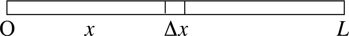
Figure 4 See Question T6.
Question T6
Figure 4 shows a thin horizontal beam of length L and uniform mass per unit length λ (i.e. the mass of the whole beam is λL).
Such a beam can be thought of as an assembly of small elements of length ∆x, each of which has a weight of magnitude λg∆x i (where g is the magnitude of the acceleration due to gravity), and exerts a torque Γ i of magnitude xλg∆x about an axis through O that is perpendicular to the plane of Figure 4. Write down an expression, involving the limit of a sum, for the magnitude of the total torque about the axis through O due to the weight of the entire beam. Rewrite this expression as a definite integral and evaluate it.
Answer T6
The torque has a magnitude Γ that is approximately given by
$\displaystyle {\it\Gamma} \approx \sum_{i=1}^n\lambda gx_i\,\Delta x_i$
So in the limit as ∆xi → 0
$\displaystyle {\it\Gamma} = \lambda g\int_0^Lx\,dx = \lambda g\left[\dfrac{x^2}{2}\right]_0^L = \dfrac{\lambda gL^2}{2}$
Thus the beam acts as though its entire mass (λL) was concentrated at its mid–point (x = L/2).
2.4 Definite integrals: the area under a graph
Figure 5 The area under the graph of an arbitrary function may be approximated by a sum of rectangles.
In the last subsection we noted in passing, when discussing Figure 3, that a definite integral can be interpreted graphically as the area under a graph. This subsection is devoted to that geometrical interpretation.
Given a function f (x) and two values of x, such as a and b with a < b (see Figure 5), it is fairly easy to see that if f (x) is never negative between a and b then
${\Large\int_a^b}f(x)\,dx$ = the area under the graph of f (x) between x = a and x = b
provided we measure the area in the scale units used on the graph’s axes and take it to mean the area below the curve but above the horizontal axis between the given limits.
The proof of this assertion follows directly from the definition of the definite integral as the limit of a sum, since each of the terms f (xi)∆xi that appear in the sum ${\large\int}_{i=1}^nf(x_i)\Delta x_i$ provides an approximate value for the area of one of the vertical strips shown in Figure 5, and their sum approximates the total area of all the strips. In the limit, when the sum becomes the definite integral from a to b, the approximation becomes exact.
The situation is a little more complicated if a > b, or if f (x) is negative between those limits since we then have to take care over signs. Different authors deal with this problem in different ways and there is therefore considerable confusion over terminology. However, in FLAP the convention is clear:
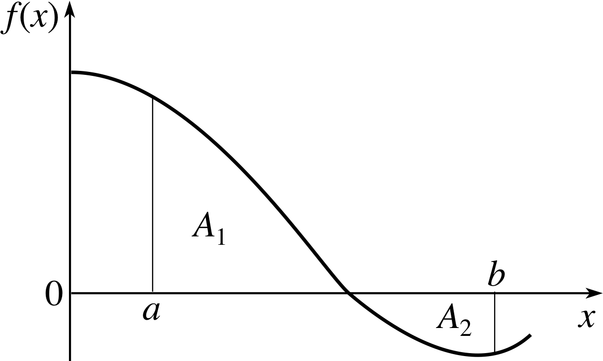
Figure 6 The area under a graph in any region where the graph is below the horizontal axis, such as A2, will be negative.
The area_under_a_grapharea under the graph of a function f (x) between x = a and x = b is equal to the corresponding definite integral,
${\large\int}_a^bf(x)\,dx = F(b) - F(a)$
It is a consequence of this definition that if, as in Figure 6, a < b, but part of the graph is below the horizontal axis, then the area under the graph in that region will be a negative quantity. i
When calculating the area under a graph between a and b, with a < b, any regions that are below the horizontal axis should be regarded as having negative areas.
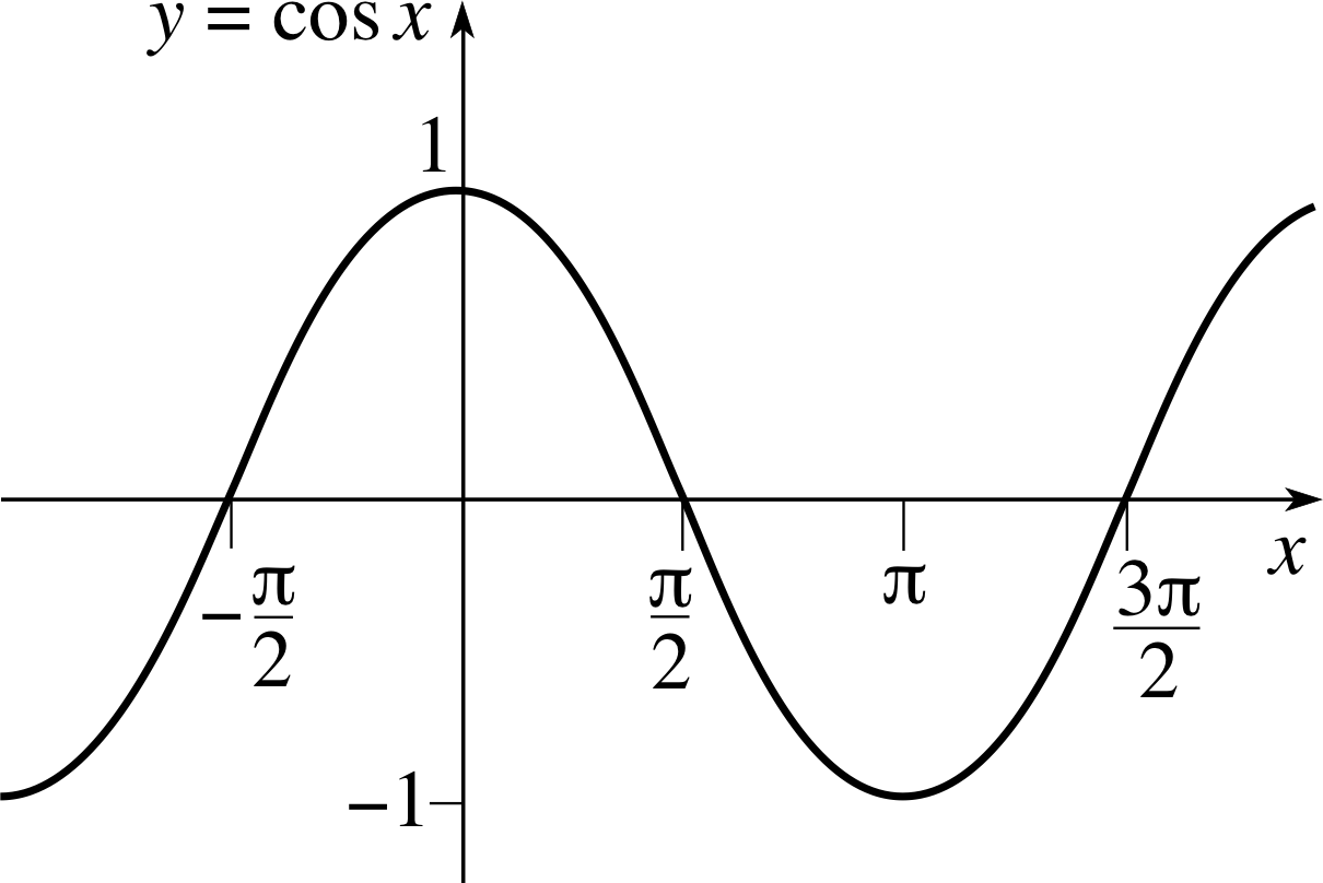
Figure 7 The graph of the function cos x.
✦ Find the area under the graph of y = cos x (Figure 7) in each of the following cases:
(a) between x = 0 and x = π/2;
(b) between x = π/2 and x = π;
(c) between x = 0 and x = π;
(d) between x = π/2 and x = 0.
✧ (a) In this case the area under the graph is
${\Large\int}_0^{\pi/2}\cos(x)\,dx = \left[\sin(x)\right]_0^{\pi/2} = \sin(\pi/2) - \sin(0) = 1$
(b) In this case the area under the graph is
${\Large\int}_{\pi/2}^\pi\cos(x)\,dx = \left[\sin(x)\right]_{\pi/2}^\pi = \sin(\pi) - \sin(\pi/2) = -1$
(c) In this case the area under the graph is
${\Large\int}_0^\pi\cos(x)\,dx = \left[\sin(x)\right]_0^\pi = \sin(\pi) - \sin(0) = 0$
(d) In this case the area under the graph is
${\Large\int}_{\pi/2}^0\cos(x)\,dx = \left[\sin(x)\right]_{\pi/2}^0 = \sin(0) - \sin(\pi/2) = -1$ i
In various problems you may be required to determine the (positive) area enclosed between various parts of the graph of f (x) and the horizontal axis, between given limits. We will indicate this by asking for the sum of the magnitudes of the enclosed areas. Since a magnitude is always a positive quantity this terminology should avoid any ambiguity. In order to determine such magnitudes you will need to consider separately each of the regions in which f (x) has a particular sign (+ or −). Thus, the sum of the magnitudes of the various regions enclosed between the graph of y = cos(x) and the x–axis, between 0 and π, is
$\displaystyle \left\lvert\,\int_0^{\pi/2}\cos(x)\,dx\,\right\rvert + \left\lvert\,\int_{\pi/2}^\pi\cos(x)\,dx\,\right\rvert = |\,1\,| + |\,-1\,| = 2$
This ‘sum of magnitudes of enclosed areas’ obviously differs from the quantity we defined to be the ‘area under the graph between 0 and π’ (in part (c) of the last question).
Question T7
Find the sum of the magnitudes of the areas enclosed by the graph of y = bx5 and the x–axis, between x = −1 m and x = 1 m, given that b = 2 m−4.
Answer T7
The function f (x) = x5 changes sign at x = 0 and therefore the required sum is
$\left\vert{\Large\int}_{-1}^0bx^5\,dx\,\right\vert + \left\vert{\Large\int}_0^1bx^5\,dx\,\right\vert = \left\vert\left[\dfrac{bx^6}{6}\right]_{-1}^0\,\right\vert + \left\vert\left[\dfrac{bx^6}{6}\right]_0^1\,\right\vert $
$\phantom{\left\vert{\Large\int}_{-1}^0bx^5\,dx\,\right\vert + \left\vert{\Large\int}_0^1bx^5\,dx\,\right\vert } = \left[\dfrac{(2\,{\rm m}^{-4})\times(1\,{\rm m}^6)}{6}\right] + \left[\dfrac{(2\,{\rm m}^{-4})\times(1\,{\rm m}^6)}{6}\right] = \dfrac{2\,{\rm m}^2}{6} + \dfrac{2\,{\rm m}^2}{6} = \dfrac23\,{\rm m}^2$
Throughout this subsection we have concentrated on the use of definite integrals to find areas under graphs, but you should realize that the reverse process is also possible and important. If you are required to find the definite integral, between a and b with a < b, of a function whose indefinite integral you are unable to determine, you can estimate the definite integral by drawing the graph of the function and measuring the area under that graph between the given limits. When doing so it is, of course, important to remember that the area should be measured in the appropriate scale units, and that regions below the horizontal axis should be regarded as having a negative area. i
3 Integrals of simple functions
Integration, the process of analysing and evaluating definite and indefinite integrals, can be very challenging. In practice everybody who uses integration regularly remembers the indefinite integrals of a variety of basic functions (xn, sin x, exp(x), etc.) and knows where to look up the indefinite integrals of some slightly more complicated functions. They also know various rules and techniques for finding the indefinite integrals of combinations of those basic functions. This section introduces the standard integrals and the simplest rules for combining them. Some of the more complicated techniques (integration by parts, integration by substitution and the use of partial fractions) are explained elsewhere in FLAP. Physicists are increasingly making use of algebraic computing packages to carry out the task of integration, but it is still necessary to appreciate the basic results of the subject in order to understand the warnings and limitations that often attend computer evaluations.
3.1 Some standard integrals
Tables 1a and 1b list a number of functions with which you should already be familiar along with their indefinite integrals. These may be classed as standard integrals. Each of the table entries can be checked by differentiating the indefinite integral to show that it is equal to the integrand. If you are going to use calculus frequently you will need to know these integrals or at least know where you can look them up quickly. When using the tables it is important to remember the following points:
| (a) | (b) i | ||
|---|---|---|---|
| f (x) | $\int f(x)\,dx$ | f (x) | $\int f(x)\,dx$ |
| k (a constant) | kx + C | 1 | x + C |
| kxn, n ≠ −1 | $k\dfrac{x^{n+1}}{n+1}+C$ | xn, n ≠ −1 | $\dfrac{x^{n+1}}{n+1} + C$ |
| $k\dfrac1x$, x ≠ 0 | k loge | x | + C | $\dfrac1x$, x ≠ 0 | loge | x | + C |
| sin(kx) | $-\dfrac1k\cos(kx) + C$ | sin(x) | −cos(kx) + C |
| cos(kx) | $\dfrac1k\sin(kx) + C$ | cos(x) | sin(kx) + C |
| tan(kx) | $\dfrac1k\loge\left\lvert\,\sec(kx)_\os\,\right\rvert + C$ | tan(x) | loge | sec(x) | + C |
| cosec(kx) | $\dfrac1k\loge\left\lvert\,\tan\left(\dfrac{kx}{2}\right)\,\right\rvert + C$ | cosec(x) | $\loge \left\lvert\,\tan\left(\dfrac x2\right)\,\right\rvert + C$ |
| sec(kx) | $\dfrac1k\loge \left\lvert\,\sec(kx)_\os + \tan(kx)\,\right\rvert + C$ | sec(x) | loge | sec(x) + tan(x) | + C |
| cot(kx) | $\dfrac1k\loge\left\lvert\,\sin(kx)_{\os}\,\right\rvert + C$ | cot(x) | loge | sin(x) | + C |
| sec2(kx) | $\dfrac1k\tan(kx) + C$ | sec2(x) | tan(x) + C |
| ekx | $\dfrac1k{\rm e}^{kx} + C$ | ex | ex + C |
| loge(kx) | x loge(kx) − x + C | loge(x) | x loge(x) − x + C |
- n and k are (given) constants and C is an arbitrary constant.
- The functions in Table 1b are special cases of those in Table 1a, corresponding to k = 1.
- In each of the trigonometric functions, x must be an angle in radians or a dimensionless real variable.
If you are reasonably proficient at differentiation many of the entries in Table 1 should come as no surprise. Indeed, we have used some of them earlier in the module on this assumption. The integrals of the reciprocal trigonometric functions (cosec, sec and cot) may seem a bit strange, but they are rarely encountered in most fields of physics so we will not dwell on them here. Far more common, and definitely worth dwelling on, is the integral of 1/x. As you can see it has been listed as loge| x | + C; the use of the modulus, | x |, should remind you that the argument of the logarithmic function must be positive, but it also indicates that the result holds true even when x itself is negative.
✦ Using Table 1 find the following
(a) ${\large\int}\,dx$, (b) ${\large\int}x^4\,dx$, (c) ${\large\int}_0^2x^4\,dx$, (d) ${\large\int}_{-2}^2x^4\,dx$, (e) ${\large\int}t^4\,dt$, (f) ${\large\int}_{-2}^2t^4\,dt$, (g) $\displaystyle \int_1^2\dfrac{dx}{x}$
✧ (a) ${\large\int}\,dx = {\large\int}1\,dx = x + C$ from Table 1b.
(b) With n = 4 the result for xn in Table 1b gives
${\Large\int}x^4\,dx = \dfrac{x^5}{5} + C$
(c) $\displaystyle \int_0^2x^4\,dx = \left[\dfrac{x^5}{5} + C\right]_0^2 = \dfrac{2^5}{5} - 0 = \dfrac{32}{5}$
(d) $\displaystyle \int_{-2}^2x^4\,dx = \left[\dfrac{x^5}{5} + C\right]_{-2}^2 = \dfrac{32}{5} - \left(\dfrac{-32}{5}\right) = \dfrac{64}{5}$
Now t and x are just dummy variables so that the results for parts (e) and (f) are identical to those of parts (b) and (d), respectively:
(e) $\dfrac{x^5}{5} + C$
(f) $\dfrac{32}{5} - \left(\dfrac{-32}{5}\right) = \dfrac{64}{5}$
(g) $\displaystyle \int_1^2\dfrac{dx}{x} = \left[\loge x\right]_1^2 = \loge 2 - \loge 1 = \loge 2 \approx 0.69$
i
✦ By differentiating the given indefinite integrals, confirm the correctness of the table entries for (a) ekx and (b) loge(kx).
✧ (a) $\dfrac{d}{dx}\left(\dfrac1k{\rm e}^{kx} + c\right) = \dfrac kk{\rm e}^{kx} = {\rm e}^{kx}$
(b) Using the product rule of differentiation
$\dfrac{d}{dx}\left[x\loge (kx) - x + C\right]\,dx = \loge (kx)\dfrac{d}{dx}(x) + x\dfrac{d}{dx}\left[\loge (kx)\right] - 1$
and remembering that
$\dfrac{d}{dx}\left[\loge (kx)\right] = \dfrac{d}{dx}\left(\loge k + \loge x\right) = \dfrac{d}{dx}\left(\loge x\right) = \dfrac1x$
we find
$\dfrac{d}{dx}\left[x\loge (kx) - x + C\right] = \loge (kx) + x\dfrac1x- 1 = \loge (kx)$
Question T8
Using Table 1 find:
(a) ${\large\int}8x^{-1}\,dx$, (b) ${\large\int}_1^38x^{-1}\,dx$, (c) ${\large\int}\sec^2(4x)\,dx$, (d) ${\large\int}_0^{\pi/16}\sec^2(4x)\,dx$
Answer T8
(a) From Table 1 ${\large\int}kx^{-1}\,dx = k\loge \vert\,x\,\vert + C$
So${\large\int}8x^{-1}\,dx = 8\loge \vert\,x\,\vert + C$
(b) ${\large\int}_1^38x^{-1}\,dx = 8\left[\loge \vert\,x\,\vert\right]_1^3 = 8\left(\loge \vert\,3\,\vert\right) - 8\left(\loge \vert\,1\,\vert\right) = 8\left[\loge (3)\right] - 8\left[\loge (1)\right] = 8\loge (3) \approx 8.789$
(c) ${\large\int}\sec^2(4x)\,dx =\frac14\tan(4x) + C$
(d) ${\large\int}_0^{\pi/16}\sec^2(4x)\,dx =\left[\dfrac14\tan(4x)\right]_0^{\pi/16} = \left(\dfrac14\tan\dfrac{\pi}{4}\right) - 0 = \dfrac14$
The following question illustrates how such calculations may arise in physics.
✦ In Subsection 2.3 we discussed the expansion of a gas in a cylinder and we showed that W, the work done by the gas as it expands, can be expressed in the form
$W = {\Large\int}_{V_a}^{V_b}P(V)\,dV$
The exact form of the function P (V) depends on the nature of the gas, but for a fixed quantity of ideal gas, expanding at a fixed temperature
$P(V) = \dfrac AV$ for some constant A i
and hence $W = {\Large\int}_{V_a}^{V_b}\dfrac AV\,dV$
Evaluate W for such a gas, in terms of Va and Vb.
✧ $W = {\Large\int}_{V_a}^{V_b}\dfrac AV\,dV = A\left[\loge \vert\,V_\os\,\vert\right]_{V_a}^{V_b}$ i
i.e.$W = \left[\loge (V_b) - \loge (V_a)\right] = A\loge (V_b/V_a)$ i
Note that in the final answer for W, the argument of the logarithmic function is dimensionless. This must always be the case in any kind of physical calculation. After all, it makes sense to write loge(6) but what sense could be made of loge(6 m) or loge(6 kg)? It is worth noting in this context that the process of integration may sometimes lead you to expressions of the kind loge(x) + C, where x is a quantity that has dimensions. When this happens you can recover a dimensionless argument by writing the constant of integration in the form −logeD, for an appropriate constant D, and then using the identity
logex − logeD = loge(x/D)
The argument is then dimensionless, providing x and D have the same dimensions.
3.2 Combining integrals
Very seldom do we have functions to integrate which are exactly those listed in Table 1. The useful general results which follow allow us much more flexibility.
Integrating the sum of two functions
Suppose that we wish to obtain an indefinite integral of the function
f (x) = 4x3 + 2x
The function x4 has a derivative 4x3, and the function x2 has a derivative 2x, so that the function x4 + x2 has a derivative 4x3 + 2x. Hence
${\large\int}(4x^3 + 2x)\,dx = x^4 + x^2 + C$
Note the appearance of only one constant of integration. Also note that the integral of the sum is a sum of the indefinite integrals of the terms in the sum. This is a particular case of a general rule:
the sum_rule_for_integrationsum rule ${\large\int}\left[g(x) + h(x)\right]\,dx = {\large\int}g(x)\,dx + {\large\int}h(x\,)dx$(14)
(With the proviso that only one constant of integration is needed on the right.)
✦ Find the following integrals:
(a) ${\large\int}(\sin x + \cos x)\,dx$, (b) ${\large\int_0^{\pi/2}}(\sin x + \cos x)\,dx$
✧ Using Table 1 we obtain:
(a) $\int(\sin x + \cos x)\,dx = -\cos x + \sin x + C$
(b) ${\Large\int}_0^{\pi/2}\left[\sin x + \cos x\right]\,dx = \left[-\cos x + \sin x\right]_0^{\pi/2}$ i
(b) $= \left(-\cos\pi + \sin\pi\right) - (-\cos0 + \sin0) = (-0 + 1) - (-1 + 0) = 1 + 1 = 2$
Integrating a constant multiple of a function
Another general rule for integrating combinations, albeit of a rather trivial sort, is given by the following constant multiple rule:
the constant_multiple_rule_for_integrationconstant multiple rule ${\large\int}kf(x)\,dx = k{\large\int}f(x\,)dx$(15)
This result has already been used in several places without comment.
Integrating a linear combination of functions
A linear combination of two functions f (x) and g (x) is a function of the form kf (x) + lg (x) where k and l are constants. We can find a general rule for integrating such combinations by combining the last two results (given in Equations 14 and 15)
${\large\int}\left[kf(x) + lg(x)\right]\,dx = k{\large\int}f(x)\,dx + l{\large\int}g(x\,)dx$(16)
✦ Using Table 1 and Equation 16 evaluate the following:
(a) ${\large\int}\left[6\cos(x) - 2\sin(x)\right]dx$, (b) ${\large\int}_{\pi/4}^{\pi/2}\left[6\cos(x) - 2\sin(x)\right]dx$
✧ (a) ${\Large\int}\left[6\cos(x) - 2\sin(x)\right]\,dx = 6\sin(x) + 2\cos(x) + C$
(b) ${\Large\int}_{\pi/4}^{\pi/2}\left[6\cos(x) - 2\sin(x)\right]\,dx = \left[6\sin(x) + 2\cos(x)\right]_{\pi/4}^{\pi/2}$
(b) $= \left(6\sin\dfrac{\pi}{2} + \cos\dfrac{\pi}{2}\right) - \left(6\sin\dfrac{\pi}{4} + \cos\dfrac{\pi}{4}\right) = (6+0) - \left(\dfrac{6}{\sqrt{2\os}}+ \dfrac{2}{\sqrt{2\os}}\right) = 6 - \dfrac{8}{\sqrt{2\os}} \approx 0.343$
Question T9
Find the following integrals:
(a) ${\large\int}\sqrt{x\os}(x^2 - 3)\,dx$ [Hint: Expand the brackets.]
(b) $\displaystyle \int\left(\dfrac{5}{t^{2/3}} + \dfrac{2}{t^{1/3}}\right)\,dt$
(c) $\displaystyle \int_1^3\dfrac{(x+2)^2}{\sqrt{x\os}}\,dx$
(d) $\displaystyle \int\dfrac{t^2-6t+1}{t^4}\,dt$
(e) ${\large\int}\left[-3\cos(x) + 2\sec^2(x)\right]\,dx$
(f) ${\large\int_0^{\pi/4}}\tan^2(\theta)\,d\theta$ [Hint: sec2(θ) = tan2(θ) + 1]
Answer T9
(a) ${\large\int}\sqrt{x\os}(x^2 - 3)\,dx = {\large\int}(x^{5/2} - 3x^{1/2})\,dx = \dfrac27x^{7/2} - 2x^{3/2} + C = \dfrac{2x\sqrt{x\os}}{7}(x^2-7) + C$
(b) $\displaystyle \int\left(\dfrac{5}{t^{2/3}} + \dfrac{2}{t^{1/3}}\right)\,dt = \int(5t^{-2/3} + 2t^{-1/3}\,dt = 15t^{1/3} + 3t^{2/3} + C$
(c) $\displaystyle \int_1^3\dfrac{(x+2)^2}{\sqrt{x\os}}\,dx = \int_1^3\dfrac{x^2+4x+4}{\sqrt{x\os}}\,dx = \int_1^3(x^{3/2}+4x^{1/2}+4x^{-1/2})\,dx = \left[\dfrac25x^{5/2} + \dfrac83x^{3/2} + 8x^{1/2}\right]_1^3$
(c) $\phantom{\displaystyle \int_1^3\dfrac{(x+2)^2}{\sqrt{x\os}}\,dx }= \left(\dfrac25\times 9\sqrt{3\os} + \dfrac83\times 3\sqrt{3\os} + 8\sqrt{3\os} \right) - \left(\dfrac25+\dfrac83+8\right) = \dfrac{98}{3}\sqrt{3\os} - \dfrac{166}{15} \approx 22.882$
(d) $\displaystyle \int\dfrac{t^2-6t+1}{t^4}\,dt = \int(t^{-2}-6t^{-4}+t^{-4})\,dt = -t^{-1} + 3t^{-2} - \dfrac13t^{-3} + C = -\dfrac1t + \dfrac{3}{t^2} - \dfrac{1}{3t^3} + C$
(e) ${\large\int}\left[-3\cos(x) + 2\sec^2(x)\right]\,dx = -3\sin(x) + 2\tan(x) + C$
(f) ${\large\int}\tan^2(\theta)\,d\theta = {\large\int}\left[\sec^2(\theta) - 1\right]\,d\theta = {\large\int}\sec^2(\theta)\,d\theta - {\large\int}1\,d\theta = \tan(\theta) - \theta + C$
therefore${\large\int}_0^{\pi/4}\tan^2(\theta)\,d\theta = \left[\tan(\theta) - \theta\right]_0^{\pi/4} = \left(1-\dfrac{\pi}{4}\right) - 0 = 1 - \dfrac{\pi}{4} \approx 0.215$
Question T10
Evaluate the integral ${\large\int}_1^2\left[\sin(\pi x) + \pi\loge (3x)\right]\,dx$
Answer T10
${\large\int}_1^2\left[\sin(\pi x) + \pi\loge (3x)\right]\,dx = \left[-\dfrac{1}{\pi}\cos(\pi x) + x\pi\loge (3x) - x\pi\right]_1^2$
$\phantom{{\large\int}_1^2\left[\sin(\pi x) + \pi\loge (3x)\right]\,dx }= \left(-\dfrac{1}{\pi}\cos(2\pi) + 2\pi\loge (6) - 2\pi\right) - \left(-\dfrac{1}{\pi}\cos(\pi) + \pi\loge (3) - \pi\right)$
$\phantom{{\large\int}_1^2\left[\sin(\pi x) + \pi\loge (3x)\right]\,dx }= \left(-\dfrac{1}{\pi} + 2\pi\loge (6) -2\pi\right) - \left(\dfrac{1}{\pi}+\pi\loge (3) - \pi\right)$
$\phantom{{\large\int}_1^2\left[\sin(\pi x) + \pi\loge (3x)\right]\,dx }= -\dfrac{2}{\pi} + \pi\loge 12 - \pi \approx 4.028\,35$
3.3 Further standard integrals
The integrals listed in Table 1 may all be classed as standard integrals, that is to say they are well known results that may be used in their own right or in the evaluation of other, more complicated, integrals. In this subsection we extend the list of standard integrals by adding the more complicated cases covered in Table 2 below. More extensive lists of standard integrals can be found in various reference works. Some of these contain hundreds of pages of integrals!
A note about inverse trigonometric functions and hyperbolic functions The inverse trigonometric functions arcsin(x), arccos(x) and arctan(x) are the inverses of the functions sin(x), cos(x) and tan(x), respectively, so that, for example arcsin(sin(θ)) = θ, provided −π/2 ≤ θ ≤ π/2. The alternative notations: sin−1(x), cos−1(x) and tan−1(x) and asin(x), acos(x) and atan(x) are also in common use.
The hyperbolic functions are defined by
$\sinh(x) = \dfrac{{\rm e}^x - {\rm e}^{-x}}{2}$ (pronounced ‘shine x’)
$\sinh(x) = \dfrac{{\rm e}^x + {\rm e}^{-x}}{2}$ (pronounced ‘cosh x’)
$\tanh(x) = \dfrac{{\rm e}^x - {\rm e}^{-x}}{{\rm e}^x + {\rm e}^{-x}}= \dfrac{\sinh(x)}{\cosh(x)}$ (pronounced ‘than x’, ‘th’ as in ‘beneath’)
Their inverses arcsinh(x), arccosh(x) and arctanh(x) are often written as sinh−1(x), cosh−1(x) and tanh−1(x).
For further information see hyperbolic functions in the Glossary.
| f (x) | $\int f(x)\,dx$ | |
|---|---|---|
| $\dfrac{1}{ax+b}$ | $\dfrac1a\loge \left\lvert\,ax+b\,\right\rvert+C$ | |
| $\dfrac{1}{b^2+a^2x^2}$ (a > 0) | $\dfrac{1}{ab}\arctan\left(\dfrac{ax}{b}\right)+C$ | |
| $\dfrac{1}{a^2x^2-b^2}$ (a > 0) | $\dfrac{1}{2ab}\loge \left\vert\dfrac{ax-b}{ax+b}\right\vert+C$ | |
| $\dfrac{1}{\sqrt{b^2+a^2x^2}}$ (a > 0) | $\dfrac1a\arcsinh\left(\dfrac{ax}{b}\right)+C = \dfrac1a\loge \left\vert \,ax+\sqrt{a^2x^2+b^2}\,\right\vert+C$ | |
| $\dfrac{1}{\sqrt{b^2-a^2x^2}}$ (a > 0) | $\dfrac1a\arcsin\left(\dfrac{ax}{b}\right)+C$ | |
| $\dfrac{1}{\sqrt{a^2x^2-b^2}}$ (a > 0) | $\dfrac1a\arccosh\left(\dfrac{ax}{b}\right)+C = \dfrac1a\loge \left\vert \,ax+\sqrt{a^2x^2-b^2}\,\right\vert+C$ | |
| $\dfrac{x}{\sqrt{b^2+a^2x^2}}$ | $\left(\dfrac{b^2}{a^2}+x^2\right)\dfrac{1}{\sqrt{b^2+a^2x^2}}+C = \dfrac{1}{a^2}\sqrt{b^2+a^2x^2}+C$ | |
| $\dfrac{x}{\sqrt{b^2-a^2x^2}}$ | $\left(-\dfrac{b^2}{a^2}+x^2\right)\dfrac{1}{\sqrt{b^2-a^2x^2}}+C = -\dfrac{1}{a^2}\sqrt{b^2-a^2x^2}+C$ | |
| $\dfrac{x}{\sqrt{a^2x^2-b^2}}$ | $\left(-\dfrac{b^2}{a^2}+x^2\right)\dfrac{1}{\sqrt{a^2x^2-b^2}}+C = -\dfrac{1}{a^2}\sqrt{a^2x^2-b^2}+C$ | |
| $\sqrt{b^2+a^2x^2}$ | $\dfrac1a\left[\dfrac12ax\sqrt{a^2x^2+b^2}+\dfrac12b^2\loge \left\vert\,ax+\sqrt{a^2x^2+b^2}\,\right\vert\right]+C$ | |
| $\sqrt{b^2-a^2x^2}$ (a > 0) | $\dfrac1a\left[\dfrac12ax\sqrt{a^2x^2+b^2}+\dfrac12b^2\arcsin\left(\dfrac{ax}{b}\right)\right]+C$ | |
| $\sqrt{a^2x^2-b^2}$ | $\dfrac1a\left[\dfrac12ax\sqrt{a^2x^2-b^2}-\dfrac12b^2\loge \left\vert\,ax+\sqrt{a^2x^2-b^2}\,\right\vert\right]+C$ | |
| exp(ax) sin(bx) | $\dfrac{\exp(ax)}{a^2+b^2}\left[a\sin(bx)-b\cos(bx)\right]+C$ | |
| exp(ax) cos(bx) | $\dfrac{\exp(ax)}{a^2+b^2}\left[a\cos(bx)+b\sin(bx)\right]+C$ |
It should be noted that several of the integrals given in Table 2 are subject to restrictions. For instance, arcsin(ax/b) is only defined for − | b/a | ≤ x ≤ | b/a |, and those expressions enclosed by square roots must be positive for all relevant values of x. We will not spell all these restrictions out in full, though we will have more to say on this topic in Subsection 4.3. However, it is important to keep your wits about you whenever you use tabulated results of this kind or the equivalent results that might be supplied by a computer program.
✦ Using Table 2, evaluate $\displaystyle \int_{-1}^1\dfrac{1}{1 + x^2}\,dx$.
✧ From Table 2, with a = b = 1, we find
$\displaystyle \int_{-1}^1\dfrac{1}{1+x}\,dx = \left[\arctan x\right]_{-1}^1 = \arctan(1) - \arctan(-1) = \dfrac{\pi}{4} - \left(\dfrac{-\pi}{4}\right) = \dfrac{\pi}{2}$
Study comment Many of the results in Table 2 can be derived by considering inverse trigonometric functions, though the derivations can be tricky and often involve the technique of implicit differentiation. We give an example of one of these derivations below (in Example 2) and then ask you to perform another for yourself. However, if you are unfamiliar with implicit differentiation you may wish to omit both and go directly to Question T11.
Example 2
Confirm by differentiation that (as implied by Table 2) the indefinite integral of $\dfrac{1}{\sqrt{1-x^2}}$ is arcsin(x) + C.
Solution
Let y = arcsin(x) then sin(y) = x and, upon differentiating both sides of this equation with respect to x, we obtain
$\cos(y)\dfrac{dy}{dx} = 1$ i
But x = sin(y), so we can use the identity sin2 (y) + cos2 (y) = 1 to write
$\cos(y) = \pm\sqrt{1-\sin^2(y)} = \pm\sqrt{1-x^2}$
where the sign ambiguity (±) has arisen because $\sqrt{x\os}$ represents a positive square root in this module.
We also know that $\dfrac{dy}{dx} = \dfrac{1}{\cos(y)}$
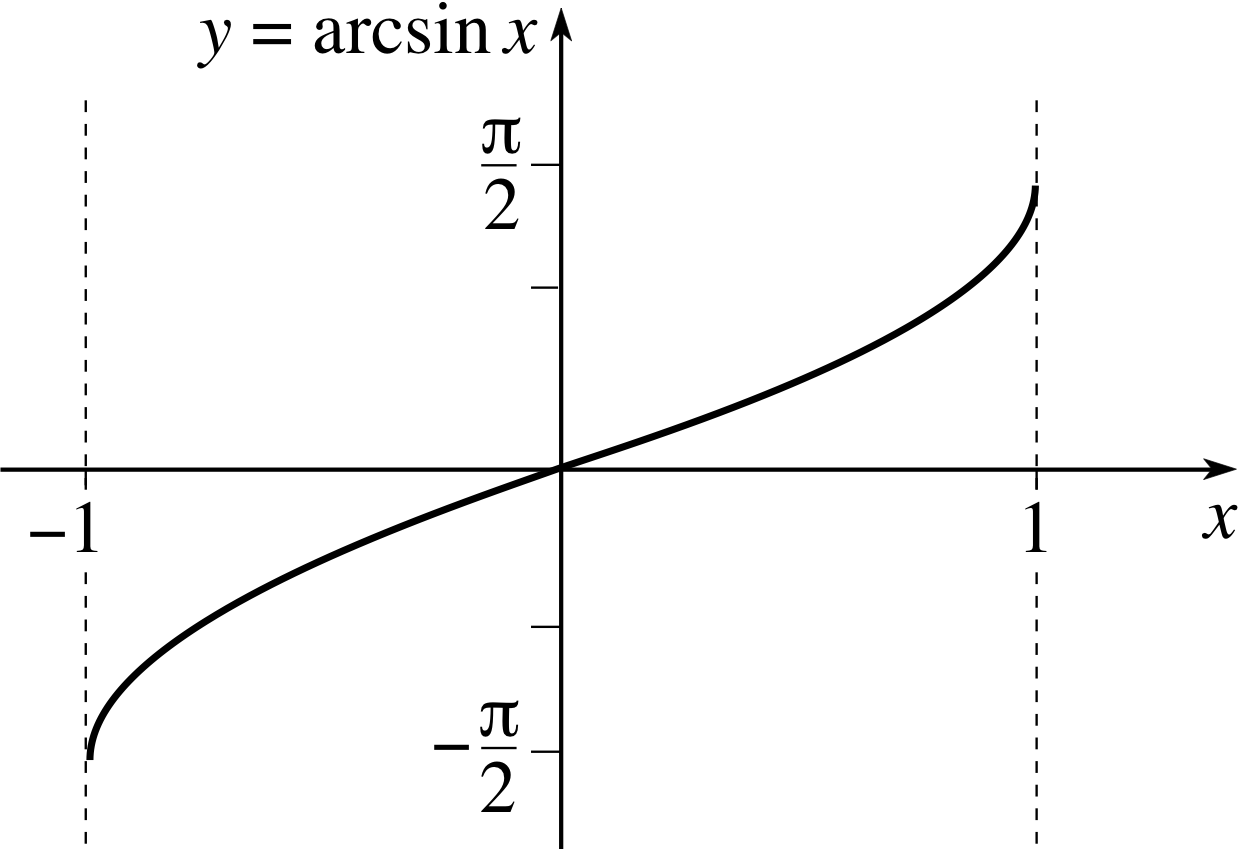
Figure 8 The graph of arcsin(x).
so,$\dfrac{dy}{dx} = \dfrac{\pm 1}{\sqrt{1-x^2}}$(17)
However, the arcsin function (see Figure 8) is conventionally defined in such a way that its gradient (i.e. its first derivative) is positive everywhere, so we must select the positive sign in Equation 17.
Thus$\dfrac{d}{dx}\left[\arcsin(x)\right] = \dfrac{1}{\sqrt{1-x^2}}$
It follows that
$\displaystyle \int\dfrac{1}{\sqrt{1-x^2}}\,dx = \arcsin(x) + C$ as implied by Table 2.
✦ Show that (as implied by Table 2) $\displaystyle \int\frac{1}{1 + x^2}\,dx = \arctan(x) + C$.
✧ Let y = arctan(x) then tan(y) = x and, differentiating both sides of the equation with respect to x, we have
$\sec^2(y)\dfrac{dy}{dx} =1$
But x = tan(y), so we can use the identity sec2(y) = 1 + tan2(y) to write
sec2(y) = 1 + tan2(y) = 1 + x2
thus$\dfrac{d}{dx}\arctan(x) = \dfrac{1}{1 + x^2}$ i
so$\displaystyle \int\dfrac{1}{1 + x^2}\,dx = \arctan(x) + C$
Question T11
Find the following integrals: 2
(a) ${\Large\int}_0^2{\rm e}^{3-2x}\,dx$ (b) $\displaystyle \int\left(\dfrac{3x+2}{x+4}\right)\,dx$ [Hint: Write 3x + 2 = 3 (x + 4) − 10]
(c) $\displaystyle \int_2^4\dfrac{1}{5x^2 + 20}\,dx$, (d) $\displaystyle \int_0^{1/3}\dfrac{3}{(8-9x^2)^{1/2}}\,dx$ i
Answer T11
(a) ${\Large\int}_0^2{\rm e}^{3-2x}\,dx = \left[-\dfrac12{\rm e}^{3-2x}\right]_0^2 = \left(-\dfrac12{\rm e}^{-1}\right) - \left(-\dfrac12{\rm e}^3\right) = \dfrac12\left({\rm e}^3 - \dfrac{1}{{\rm e}}\right)$
(b) $\displaystyle \int\left(\dfrac{3x+2}{x+4}\right)\,dx = \int\left[\dfrac{3(x+4)-10}{x+4}\right]\,dx = \int\left(3 - \dfrac{10}{x+4}\right)\,dx = 3x - 10\loge \vert\,x+4\,\vert + C$
(c) $\displaystyle \int_2^4\dfrac{1}{5x^2 + 20}\,dx = \dfrac15\int_2^4\dfrac{1}{x^2 + 4}\,dx = \left[\dfrac15\times\dfrac12\arctan\left(\dfrac x2\right)\right]_2^4$
(c) $\phantom{\displaystyle \int_2^4\dfrac{1}{5x^2 + 20}\,dx }= \left[\dfrac{1}{10}\arctan(2)-\dfrac{1}{10}\arctan(1)\right] = \dfrac{1}{10}\left[\arctan(2) - \pi/4\right]$
(d) $\displaystyle \int_0^{1/3}\dfrac{3}{(8-9x^2)^{1/2}}\,dx = \left[\arcsin\left(\dfrac{3x}{2\sqrt{2\os}}\right)\right]_0^{1/3} = \arcsin\left(\dfrac{1}{2\sqrt{2\os}}\right)$
4 More about definite integrals
4.1 Properties of definite integrals
The definite integral has the following mathematical properties, each of which makes good sense if you interpret it in terms of the (signed) area under a graph.
Properties of definite integrals:
- 1
-
${\large\int}_a^af(x)\,dx = 0$(18)
- 2
-
${\large\int}_b^af(x)\,dx = -{\large\int}_a^bf(x)\,dx$(19)
- 3
-
${\large\int}_a^bf(x)\,dx ={\large\int}_a^cf(x)\,dx + {\large\int}_c^bf(x)\,dx$ where a ≤ c ≤ b(20)
- 4
-
${\large\int}_a^b\left[kf(x) + lg(x)\right]\,dx = k{\large\int}_a^bf(x)\,dx + l{\large\int}_a^bg(x)dx$(21)
- 5
-
If f (x) ≥ 0 for all x in the interval a ≤ x ≤ b then
${\large\int}_a^bf(x)\,dx \ge 0$(22)
- 6
-
If m ≤ f (x) ≤ M for all x in the interval a ≤ x ≤ b then
$m(b - a) \le {\large\int}_a^bf(x)\,dx \le M(b - a)$(23)
Properties 1 to 3 are derived below using the fundamental theorem of calculus. Property 4 is the extension to definite integrals of the rules for combining indefinite integrals that were introduced in Subsection 3.2, it too can be derived using the fundamental theorem of calculus. Properties 5 and 6 follow from the definition of a definite integral as the limit of a sum. They are not derived in this module, but they may be treated as tutorial exercises.
- 1
-
If b = a then ${\large\int}_a^af(x)\,dx = F(a) - F(a) = 0$
- 2
-
${\large\int}_b^af(x)\,dx = F(a) - F(b) = -(F(b) - F(a)) = -{\large\int}_a^bf(x)\,dx$
- 3
-
${\large\int}_a^cf(x)\,dx + {\large\int}_c^bf(x)\,dx = F(c) - F(a) - F(c) - F(b) = {\large\int}_a^bf(x)\,dx$
Property 6 can be useful in cases where it is impossible to calculate the integral exactly. In such cases it is often desirable to obtain an estimate for the integral. The following example illustrates the method:
✦ By considering the maximum and minimum values of $\sqrt{x^2+1}$ in the interval 1 ≤ x ≤ 3, show that
$2\sqrt{2\os} \le {\Large\int}_1^3\sqrt{x^2 +1}\,dx \le 2\sqrt{10\os}$
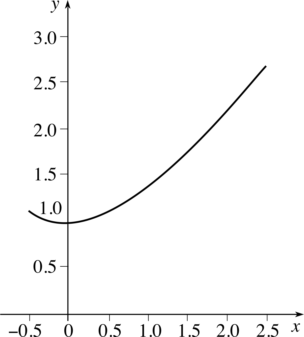
Figure 9 The graph of $y=\sqrt{x^2+1}$.
✧ Figure 9 shows the graph of $y = \sqrt{x^2+1}$. Clearly the least value of $\sqrt{x^2+1}$ in the given interval is $\sqrt{2\os}$ (when x = 1) and the greatest value is $\sqrt{10\os}$ (when x = 3). Thus, from Property 6,
If m ≤ f (x) ≤ M for all x in the interval a ≤ x ≤ b then
$m(b - a) \le {\Large\int}_a^bf(x)\,dx \le M(b - a)$(Eqn 23)
we have
$2\sqrt{2\os} \le {\Large\int}_1^3\sqrt{x^2+1}\,dx \le 2\sqrt{10\os}$
Question T12
If f (x) ≥ g (x) for all x where a ≤ x ≤ b show that
${\large\int}_a^b f(x)\,dx \ge {\large\int}_a^bg(x)\,dx$
[Hint: Consider f (x) − g (x).]
Answer T12
By Property 5,
If f (x) ≥ 0 for all x in the interval a ≤ x ≤ b then ${\large\int}_a^bf (x)\,dx \ge 0$(Eqn 22)
${\Large\int}_a^b[f(x) - g(x)]\,dx \ge 0$
i.e.${\Large\int}_a^bf(x)\,dx - {\Large\int}_a^bg(x)\,dx \ge 0$
Hence the result ${\Large\int}_a^bf(x)\,dx \ge {\Large\int}_a^bg(x)\,dx$
Question T13
A bullet of mass m is fired horizontally into a box full of sand. As the bullet travels through the sand its motion is opposed by a resistive force of magnitude
$F(x) = \sqrt[{\large\raise{2pt}3}]{(a^3 - b^3x^3)}m$
where a and b are positive constants, and x is the distance the bullet has travelled through the sand. In a particular test, it is found that the bullet travels a distance L = a/b through the sand before being brought to rest.
Using an appropriate limit of a sum, write down an expression for the work done in bringing the bullet to rest. Rewrite your answer as a definite integral, but do not attempt to evaluate it. Given that the work done in bringing the bullet to rest is equal to minus the initial kinetic energy of the bullet when it enters the sand, write down an upper estimate of that initial kinetic energy, in terms of a, b, and m.
[Hint: The work done when a force constant force Fx moves its point of application through a displacement ∆x is generally ∆W = Fx ∆x. In this case the force is variable, and only its magnitude is given, but the fact that it brings the bullet to rest shows that it acts in the opposite direction to the displacement and therefore does a negative amount of work.]
Answer T13
The work done is given by
$\displaystyle W = \lim_{\Delta x\rightarrow 0}\left(\sum_{i=1}^n-F(x_i)\Delta x_i\right)$
where x1 = 0, xn+1 = a/b, and ∆x represents the largest of the ∆xi which are themselves defined by ∆xi = xi+1 − xi,
with x1 < x2 < x3 ... < xn−1 < xn < xn+1.
It follows from this definition that
$\displaystyle W = \int_0^{a/b}-F(x)\,dx = -\int_0^{a/b}F(x)\,dx$
Since the initial kinetic energy is minus the work done by the resistive force in bringing the bullet to rest,
initial kinetic energy = $\displaystyle \int_0^{a/b}F(x)\,dx = \int_0^{a/b}\sqrt[{\large\raise{2pt}3}]{(a^3-b^3x^3)}m\,dx$
The greatest value of $\sqrt[{\large\raise{2pt}3}]{(a^3-b^3x^3)}m$ in the interval 0 ≤ x ≤ a/b occurs at x = 0, so that by Property 6:
If m ≤ f (x) ≤ M for all x in the interval a ≤ x ≤ b then $m(b - a) \le {\large\int}_a^bf(x)\,dx \le M(b - a)$(Eqn 23)
$\displaystyle \int_0^{a/b}\sqrt[{\large\raise{2pt}3}]{(a^3-b^3x^3)}m\,dx \le \sqrt[{\large\raise{2pt}3}]{a^3}m \times \dfrac ab = \dfrac{ma^2}{b}$
4.2 Odd, even and periodic integrands
Odd and even functions
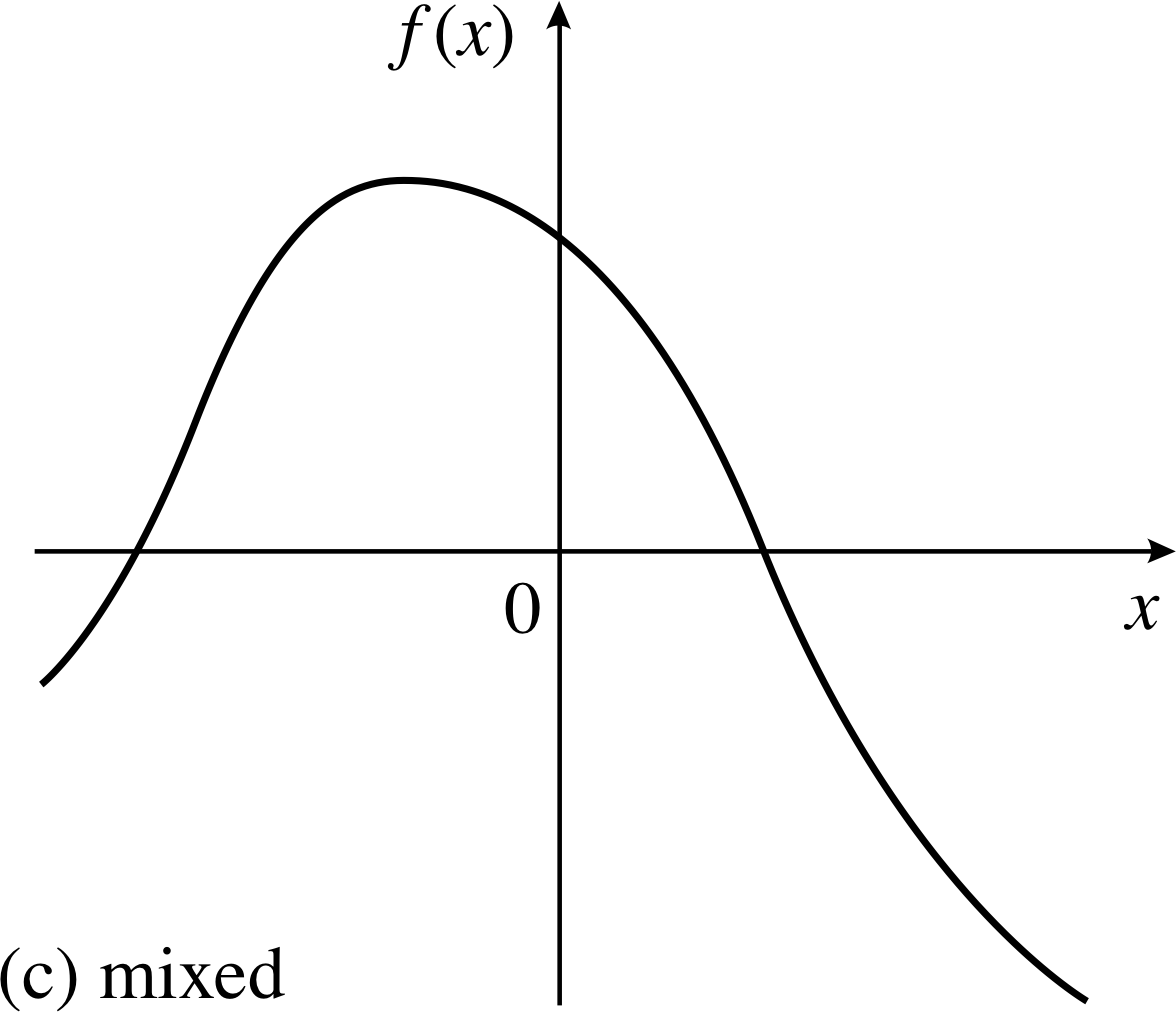
Figure 10 (c) A function of mixed symmetry.
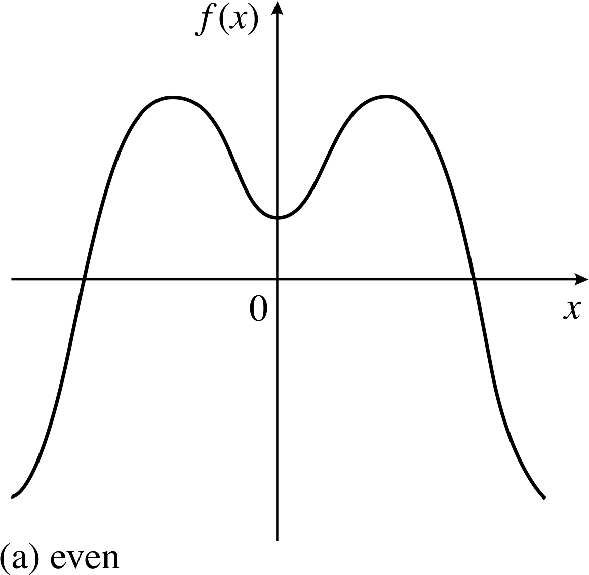
Figure 10 (a) An even function.
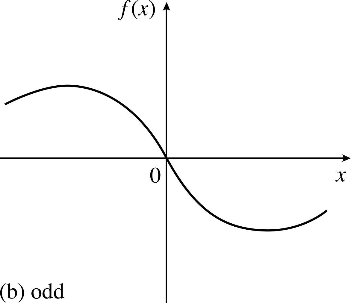
Figure 10 (b) An odd function.
When looking at the graphs of functions it is easy to see that some functions are symmetric about a vertical line through the origin and others are not. Three examples of this are shown in Figure 10. Part (a) of the figure shows a function f (x) that is obviously symmetric about the origin – the part of the graph drawn to the left of the origin is the mirror image of the part to the right of the origin. Mathematically, such a function is called an even function and is characterized by the property
f (−x) = f (x) for all x in the domain of f (x) (even function)
Even functions are sometimes referred to as symmetric functions.
Figure 10b shows a different function. It certainly isn’t an even function yet there is clearly some sort of relationship between the parts of the function shown to the left of the origin and those to the right. Functions of this sort are called odd functions and are characterized by the property
f (−x) = −f (x) for all x in the domain of f (x) (odd function)
Odd functions are sometimes referred to as antisymmetric functions.
Figure 10c shows a function f (x) which is neither odd nor even. There is no simple relationship between f (−x) and f (x) for this function, though it is interesting (and occasionally useful) to note that any function with a symmetric domain, i including this one, can be written as the sum of an even function and an odd function. To see why this is so consider the following identity which holds true for any function f (x)
f (x) = ½ [f (x) + f (−x)] + ½ [f (x) − f (−x)](24)
The first term on the right–hand side of this identity, [f (x) + f (−x)]/2, is an even function as you can see if you replace x by −x everywhere within it; and, by the same argument, the second term, [f (x) − f (−x)]/2, is an odd function. Thus, an arbitrary function can indeed be written as a sum of even and odd parts. Functions which are neither purely even nor purely odd are sometimes referred to as functions of mixed symmetry.
✦ Classify each of the following functions as even, odd or of mixed symmetry:
(a) x3 (b) 2x + 4x4 + 1 (c) sin(x) (d) 2 cos(3x)
✧ (a) If f (x) = x3, then
f (−x) = (−x)3 = −x3 = −f (x)
So x3 is an odd function of x.
(b) Similarly, if f (x) = 2x + 4x4 + 1, then
f (−x) = 2 (−x) + 4 (−x)4 + 1 = −2x + 4x4 + 1
which is neither f (x) nor −f (x), so 2x + 4x4 + 1 is of mixed symmetry.
(c) sin(−x) = −sin(x), so sin(x) is an odd function.
(d) 2 cos(−3x) = 2 cos(3x), so 2 cos(3x) is an even function. i
The examples we have just considered have been fairly straightforward. In more complicated cases involving the products of two or more functions it is often useful to recall the following rules:
even function × even function = even function
odd function × odd function = even function
odd function × even function = odd function
These are similar to the rules for products of signs.
Integrals of even and odd functions
If you think of a definite integral in terms of the area under a graph, then it should be clear from Figure 10 that
If f (x) is an odd function, then $\displaystyle \int_{-a}^af(x)\,dx = 0$(25)
If f (x) is an even function, then $\displaystyle \int_{-a}^af(x)\,dx = 2\int_0^af(x)\,dx$(26)
Note that in both these integrals the range of integration (from −a to a) is symmetric about the origin. Don’t expect these results to work in more general situations.
These two results can often be of help when evaluating definite integrals, especially the first result (Equation 25) which sometimes removes the need to do any hard work at all.
✦ Evaluate ${\Large\int}_{-\pi}^\pi 4x^2\sin(2x)\,dx$
✧ In this case the range of integration is symmetric about the origin and the integrand is an odd function. i Consequently, we can say that the integral is zero without any further work.
Odd and even functions arise in many fields of physics so you should always ask yourself if you can use symmetry to simplify the process of definite integration. This is especially true in quantum physics where you will often be asked to integrate functions of known symmetry. Another property of many of the functions that have to be integrated in a course on quantum physics is periodicity.
Periodic functions and their integrals
A function f (x) is said to be periodic_functionperiodic if there exists a constant k (> 0) such that
f (x) = f (x + nk) for all x and for all integers (i.e. whole numbers) n
The smallest value of k for which this condition holds true is called the period of the function.
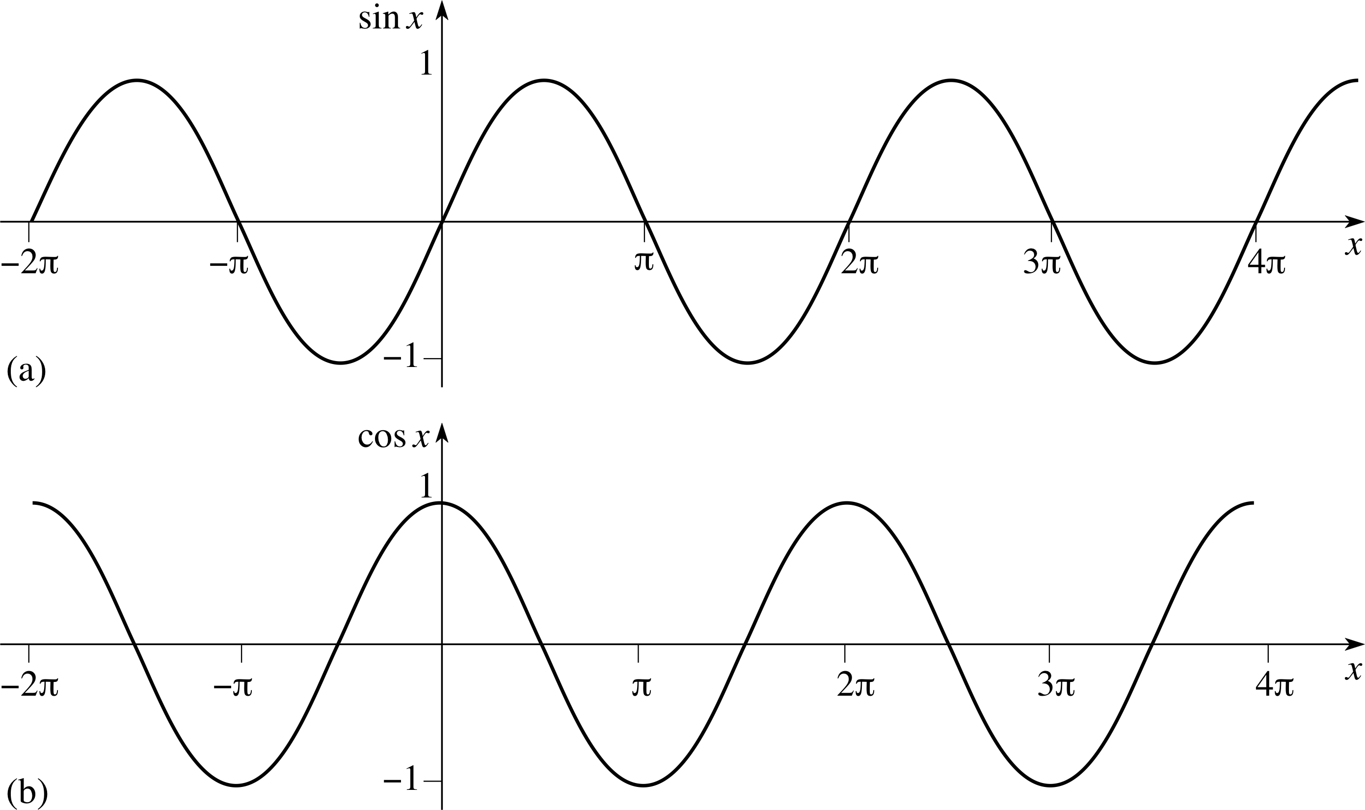
Figure 11 The graphs of the periodic functions (a) sin(x), and (b) cos(x).
The most obvious examples of periodic functions are the trigonometric functions sin(x) and cos(x), both of which have period 2π, since
sin(x) = sin(x + 2nπ)
andcos(x) = cos(x + 2nπ)
The graphs of all periodic functions, like the graphs of sin(x) and cos(x) in Figure 11, consist of regular repetitions of a single basic unit that covers one period.
As a consequence of their repetitive nature we can state the following:
If f (x) is a periodic function of period k, then $\displaystyle \int_a^{a+k}f(x)\,dx = \int_0^kf(x)\,dx$(27)
and, if n is any integer, then $\displaystyle \int_0^{nk}f(x)\,dx = n\int_0^kf(x)\,dx$(28)
The essential point being made in Equations 27 and 28 is that when dealing with periodic functions we learn just as much by integrating over one full period as we do by integrating over several full periods. Moreover, if we are integrating over a full period, it doesn’t matter where that period begins, a general point a is just as good as the origin x = 0.
Question T14
Which of the following are equal to zero? Explain your answers. (This is an easy question, it should not require any long calculations but you will need to think.)
(a) ${\Large\int}_{-5}^53x\,dx$ (b) ${\Large\int}_{-\pi}^\pi\sin2(x^2)\,dx$ (c) ${\Large\int}_{3\pi}^{7\pi}\left[3\sin(3x)+\sin^3(x)\right]\,dx$
Answer T14
(a) ${\Large\int}_{-5}^53x\,dx = 0$ because the integrand is an odd function but the range of integration is symmetric about the origin.
(b) ${\Large\int}_{-\pi}^\pi\sin2(x^2)\,dx$ is non–zero because the integrand is never negative and is non–zero over at least part of the range of integration.
(c) ${\Large\int}_{3\pi}^{7\pi}\left[3\sin(3x)+\sin^3(x)\right]\,dx = 0$ because the integrand is an odd periodic function (of period 2π) that is being integrated over two full periods. Due to the periodic nature of the integrand we can take the range of integration to be symmetric about the origin, the oddness then ensures that the integral is zero.
4.3 Improper and divergent integrals
In the study of physics it is not uncommon to encounter definite integrals that involve infinity. In this subsection we consider two of the ways in which such integrals arise: integrals in which one or both of the limits tends towards infinity, and integrals in which the integrand itself tends towards infinity at some point in the range of integration. These are somewhat specialized topics that your tutor might advise you to omit at this stage.
Integration over an infinite range
Infinity (∞) is not a real number, so strictly speaking we cannot use it as one of the limits of integration that we introduced earlier when discussing the limit of a sum. However, you will often see integrals with an infinite upper or lower limit. Such usage is justified by the following definitions
$\displaystyle \int_{-\infty}^bf(x)\,dx = \lim_{a\rightarrow -\infty}{\left(\int_{a}^bf(x)\,dx\right)}$(29)
$\displaystyle \int_a^{\infty}f(x)\,dx = \lim_{b\rightarrow\infty}{\left(\int_{a}^bf(x)\,dx\right)}$(30)
The integrals on the left are called improper integrals. Although written as definite integrals they are not properly defined by the usual process of taking the limit of a sum; rather one or more additional limits must be taken (as indicated on the right).
If the limits on the right exist and are finite the corresponding improper integral is said to be convergent_integralconvergent. If the relevant limit does not exist, or if it tends to ±∞, then the improper integral is said to be divergent_integraldivergent.
It is easy to find divergent integrals, for example consider the following:
$\displaystyle \int_0^\infty\cos(x)\,dx = \lim_{b\rightarrow\infty}{\left(\int_a^b\cos(x)\,dx\right)} = \lim_{b\rightarrow\infty}{\left(\left[\sin(x)\right]_0^\infty\right)} = \lim_{b\rightarrow\infty}{\left[\sin(b)\right]}$
In this case the integral diverges because as b tends to infinity the value of sin(b) oscillates between 1 and −1, there is no unique limiting value, so the limit does not exist.
On the other hand, it is equally easy to find integrals that converge. For instance, if we ignore all forces other than the Earth’s gravitational pull, the minimum launch speed v that will just allow an object of fixed mass m to escape from the surface of the Earth to a point infinitely far away (i.e. the escape speed from the Earth) is given by
$\displaystyle \dfrac12mv^2 = \int_R^\infty\dfrac{GmM}{r^2}\,dr = \left[-\dfrac{GmM}{r}\right]_R^\infty = (0) - \left(-\dfrac{GmM}{R}\right) = \dfrac{GmM}{R}$ so $v = \sqrt{\dfrac{2GM}{R}}$
where G is the gravitational constant, M is the mass of the Earth and R is the radius of the Earth.
In this case the improper integral converges, and, as is customary in such cases, we have omitted the formal step of writing down the limits that are required to define properly that integral. In effect we have treated infinity as though it were a very large real number.
Improper integrals must always be treated with care and generally require case by case consideration. However, one general rule which it is useful to keep in mind is the following:
If $I = {\Large\int}f(x)\,dx$ where f (x) is continuous over the range of integration, and if, for large values of x,
$f(x) = \dfrac{g(x)}{x^n}$ where g (x) is finite and non-zero, and n > 1,
then the integral I is convergent.
Integration with an infinite integrand
The expression $\dfrac{1}{\sqrt{1-x^2}}$ is well defined only if −1 < x < 1, yet it is not unusual to see integrals such as
$\displaystyle I = \int_0^1\dfrac{1}{\sqrt{1 - x^2}}\,dx$ or $\displaystyle I = \int_{-1}^0\dfrac{1}{\sqrt{1 - x^2}}\,dx$ or even $\displaystyle I = \int_{-1}^1\dfrac{1}{\sqrt{1 - x^2}}\,dx$
What can such integrals mean when the integrand isn’t even defined at all points in the range of integration? In fact, they are all improper integrals which can be interpreted as limits of properly defined definite integrals. For example,
$\displaystyle I = \int_0^1\dfrac{1}{\sqrt{1 - x^2}}\,dx = \lim_{\varepsilon\rightarrow 0}{\left(\int_0^{1-\varepsilon}\dfrac{1}{\sqrt{1 - x^2}}\,dx\right)}$
where $\displaystyle \raise{0.5em}{\lim_{\varepsilon\rightarrow 0}}$ indicates that we are considering the limit as the positive quantity ε tends to zero, i.e. as b, the upper limit, tends to 1 from below.
With this understanding, the integrand is one of the standard integrands listed in Table 2, so we can use the corresponding indefinite integral given in that table to write
$\displaystyle I = \int_0^1\dfrac{1}{\sqrt{1 - x^2}}\,dx = \lim_{\varepsilon\rightarrow 0}{\left(\left[\arcsin x\right]_0^{1-\varepsilon}\right)} = \lim_{\varepsilon\rightarrow 0}\left[\arcsin(1-\varepsilon)\right] - (\arcsin 0) = \arcsin(1) = \dfrac{\pi}{2}$
In this case the improper integral is convergent and gives a sensible answer that can, as usual, be interpreted as (the limit of) an area under a graph, even though the graph itself cannot be drawn at x = 1.
✦ Without using the formal notation of limits, evaluate the following improper integrals:
(a) $\displaystyle I = \int_{-1}^0\dfrac{1}{\sqrt{1 - x^2}}\,dx$ (b) $\displaystyle I = \int_{-1}^1\dfrac{1}{\sqrt{1 - x^2}}\,dx$
✧ (a) $I = \displaystyle \int_{-1}^0\dfrac{1}{\sqrt{1-x^2}}\,dx = \left[\arcsin x\right]_{-1}^0 = \left[\arcsin(0)\right] - \left[\arcsin(-1)\right] = \dfrac{\pi}{2}$
(b) $I = \displaystyle \int_{-1}^1\dfrac{1}{\sqrt{1-x^2}}\,dx = \left[\arcsin x\right]_{-1}^1 = \left[\arcsin(1)\right] - \left[\arcsin(-1)\right] = \pi$ i
Although we have just considered a convergent integral it is easy to find divergent cases.
For example $\displaystyle \int_0^1\dfrac1x\,dx$ is divergent because
$\displaystyle \int_0^1\dfrac1x\,dx = \lim_{\varepsilon\rightarrow 0}{\left(\left[\loge \left\lvert\,x\,\right\rvert\right]_\varepsilon^1\right)} = \lim_{\varepsilon\rightarrow 0}{\left(0-\loge \varepsilon\right)}$ i
and log ε has no finite limit as ε tends to zero. Similarly, the integral $\displaystyle \int_0^2\dfrac{1}{(1- x)^2}\,dx$ is divergent because of the behaviour of the integrand as x tends to 1. As a general rule:
If $\displaystyle I = \int_a^\infty f(x)\,dx$ where f (x) can be written as $f(x) = \dfrac{g(x)}{(x - p)^n}$ with g (x) finite over the range of integration and non–zero at x = p, then there is said to be a singularity (or an infinity) of order_of_a_singularityorder n at x = p and the integral I is convergent if the order of that singularity is less than 1 (i.e. n < 1).
One final warning about integrals that involve a singularity, remember that even if they are written to look like ordinary definite integrals they are still improper and should be considered (at least in the back of your mind) as limits of proper integrals. Forget this and you may make the following kind of mistake:
$\displaystyle \int_{-1}^1\dfrac{1}{x^2}\,dx = \left[-\dfrac1x\right]_{-1}^1 = (-1) - (1) = -2$ (WRONG!)
It looks plausible, but there is a singularity in the middle of the range of integration. By considering the separate limits as x tends to zero from above and below it is easy to see that the integral is actually divergent.
Question T15
Rewrite the improper integral $\displaystyle \int_{-1}^1\dfrac1x\,dx$ as the sum of the limits of two properly defined definite integrals. Will it be convergent? If so, what is its value?
Answer T15
$\displaystyle \int_{-1}^1\dfrac1x\,dx = \lim_{\delta\rightarrow 0}\left(\int_{-1}^{-\delta}\dfrac1x\,dx\right) + \lim_{\varepsilon\rightarrow 0}\left(\int_\varepsilon^1\dfrac1x\,dx\right)$
where δ and ε are positive quantities. (Note that δ and ε are independent quantities, it would be wrong to use the same variable in both limits.) Thus
$\displaystyle \int_{-1}^1\dfrac1x\,dx = \lim_{\delta\rightarrow 0}\left(\left[\loge \left\vert\,x\,\right\vert\right]_{-1}^{-\delta}\right) + \lim_{\varepsilon\rightarrow 0}\left(\left[\loge \left\vert\,x\,\right\vert\right]_\varepsilon^1\right) = \lim_{\delta\rightarrow 0}\left(\loge \delta\right) + \lim_{\varepsilon\rightarrow 0}\left(-\loge \varepsilon\right)$
but neither of these limits exists, so the integral is divergent.
If we consider the following joint limit
$\displaystyle \lim_{\varepsilon\rightarrow 0}\left(\int_{-\varepsilon}^{-1}\dfrac1x\,dx + \int_\varepsilon^1\dfrac1x\,dx\right) = \lim_{\varepsilon\rightarrow 0}\left(\left[\loge \left\vert\,x\,\right\vert\right]_{-1}^{-\varepsilon} + \left[\loge \left\vert\,x\,\right\vert\right]_\varepsilon^1\right) = \lim_{\varepsilon\rightarrow 0}(\loge \varepsilon - \loge \varepsilon) = 0$
we can see that it is possible to associate a finite value with this particular improper integral, even though it is formally divergent. The value obtained by this particular kind of limiting process is called the Cauchy principal value of the integral. Such principal values are sometimes of interest, but their consideration is beyond the scope of this module.
5 Closing items
5.1 Module summary
- 1
-
A function f is a rule that assigns a single value f (x) to each value of x in a set called the domain.
- 2
-
If f (x) is a given function and F (x) is any function such that
$\dfrac{dF}{dx} = f(x)$ then we write $F(x) = {\large\int}f(x)\,dx$
and we call F (x) an Subsection 2.2indefinite integral of f (x).
- 3
-
If F1(x) and F2(x) are both indefinite integrals of the same function f (x), then there exists a constant K such that F1(x) = F2(x) + K.
- 4
-
The Subsection 2.3definite integral of a function f (x) from x = a to x = b is defined by the limit of a sum and may be written as
$\displaystyle \int_a^bf(x)\,dx = \lim_{\Delta x\rightarrow 0}{\left(\sum f(x_i)\Delta x_i\right)}$
where ∆xi = xi+1 − xi with x1 = a and xn+1 = b, and ∆x is the largest of the ∆xi.
- 5
-
According to the fundamental theorem of calculus, if F (x) is any indefinite integral of a given function f (x), such that ${\large\int}f(x)\,dx = F(x)$, then
${\large\int}_a^bf(x)\,dx = F(b) - F(a)$(Eqn 13)
- 6
-
The (signed) Subsection 2.4area under the graph of a function f (x) between x = a and x = b is equal to the corresponding definite integral, ${\large\int}_a^bf(x)\,dx = F(b) - F(a)$. When calculating the area under a graph between a and b, with a < b, any regions that are below the horizontal axis should be regarded as having negative areas.
- 7
-
Several (indefinite) Subsection 3.1standard integrals are listed in Table 1Tables 1 and Table 22.
- 8
-
Integrals (both definite and indefinite) may be combined using the following rules:
the sum rule ${\large\int}\left[g(x) + h(x)\right]\,dx = {\large\int}g(x)\,dx + {\large\int}h(x\,)dx$(Eqn 14)
the constant multiple rule ${\large\int}kf(x)\,dx = k{\large\int}f(x\,)dx$(Eqn 15)
- 9
-
Definite integrals have the following six properties:
- 1
-
${\large\int}_a^af(x)\,dx = 0$(Eqn 18)
- 2
-
${\large\int}_b^af(x)\,dx = -{\large\int}_a^bf(x)\,dx$(Eqn 19)
- 3
-
${\large\int}_a^bf(x)\,dx ={\large\int}_a^cf(x)\,dx + {\large\int}_c^bf(x)\,dx$ where a ≤ c ≤ b(Eqn 20)
- 4
-
${\large\int}_a^b\left[kf(x) + lg(x)\right]\,dx = k{\large\int}_a^bf(x)\,dx + l{\large\int}_a^bg(x)dx$ where k and l are constants(Eqn 21)
- 5
-
If f (x) ≥ 0 for all x in the interval a ≤ x ≤ b then
-
${\large\int}_a^bf(x)\,dx \ge 0$(Eqn 22)
- 6
-
If m ≤ f (x) ≤ M for all x in the interval a ≤ x ≤ b then
$m(b - a) \le {\large\int}_a^bf(x)\,dx \le M(b - a)$(Eqn 23)
- 10
-
If f (x) is an odd function so that f (−x) = −f (x), then
$\displaystyle \int_{-a}^af(x)\,dx = 0$(Eqn 25)
If f (x) is an even function so that f (−x) = f (x), then
$\displaystyle \int_{-a}^af(x)\,dx = 2\int_0^af(x)\,dx$(Eqn 26)
If f (x) is a periodic function of period k, so that f (x) = f (x + nk), where n is any integer, then
$\displaystyle \int_a^{a+k}f(x)\,dx = \int_0^kf(x)\,dx$(Eqn 27)
$\displaystyle \int_0^{nk}f(x)\,dx = n\int_0^kf(x)\,dx$(Eqn 28)
- 11
-
Subsection 4.3Improper integrals may have infinite upper or lower limits and/or singularities in their integrands. Such integrals should be interpreted as appropriate limits of (proper) definite integrals, and may be convergent or divergent. They should be treated with care.
5.2 Achievements
Having completed this module, you should be able to:
- A1
-
Define the terms that are emboldened and flagged in the margins of the module.
- A2
-
Define an indefinite integral of a given function in terms of a process that reverses the effect of differentiation, explain the significance of the constant of integration introduced by that process, and determine a variety of indefinite integrals.
- A3
-
Define the definite integral of a given function between given limits in terms of the limit of a sum, state the fundamental theorem of calculus that relates definite and indefinite integrals, and use it to evaluate a variety of definite integrals.
- A4
-
Interpret the definite integral of a given function between given limits in terms of the area under the graph of that function between those limits (with due regard to signs).
- A5
-
Use tables of standard integrals to determine definite and indefinite integrals of the tabulated functions and of linear combinations of those functions. Also, use the techniques of differentiation to justify the entries in such tables.
- A6
-
Recognize, write down and use the general mathematical properties of definite integrals.
- A7
-
Recognize, write down and use the general mathematical properties of definite integrals with integrands that are even, odd or periodic.
- A8
-
Recognize improper integrals, determine whether or not they converge in simple cases, and evaluate those that do.
Study comment You may now wish to take the following Exit test for this module which tests these Achievements. If you prefer to study the module further before taking this test then return to the topModule contents to review some of the topics.
5.3 Exit test
Study comment Having completed this module, you should be able to answer the following questions, each of which tests one or more of the Achievements.
Question E1 (A3 and A4)
(a) What is the meaning of each of the symbols in the expression ${\Large\int}_a^bf(x)\,dx$?
(b) How may we use an indefinite integral of f (x) to evaluate the integral?
(c) Give a geometrical interpretation of the integral if f (x) > 0 for all x such that a ≤ x ≤ b.
Answer E1
(a) ∫ is the integral sign. f (x) is a function of x, called the integrand, a and b are the lower and upper limits of the integration and x is the variable of integration. The integration element dx is read as ‘with respect to x’.
(b) We find a function F (x) for which $\dfrac{dF}{dx} = f(x)$; then we evaluate F (b) − F (a).
(c) The integral could represent the area under the curve y = f (x) between the lines x = a and x = b.
(Reread Subsection 2.2Subsections 2.2, Subsection 2.32.3 and Subsection 2.42.4 if you had any difficulty with this question.)
Question E2 (A2 and A3)
Find the following integrals:
(a) $\displaystyle \int\left(x^2+\dfrac{1}{x^2}\right)\,dx$ (b) $\displaystyle \int_2^1\dfrac1x\,dx$ (c) $\displaystyle \int_{\pi/6}^{\pi/2}8\cos\left(\dfrac x2\right)\,dx$ (d) $\displaystyle \int_1^2\frac12\loge \left(\dfrac12x\right)\,dx$
Answer E2
(a) $\displaystyle \int\left(x^2+\dfrac{1}{x^2}\right)\,dx = \dfrac{x^3}{3} - \dfrac1x + C$
(b) $\displaystyle \int_2^1\dfrac1x\,dx = -\int_1^2\dfrac1x\,dx = -\left[\loge x\right]_1^2 = -(\loge 2 - \loge 1) = -\loge 2 + 0 = -\loge 2$
(c) $\displaystyle \int_{\pi/6}^{\pi/2}8\cos\left(\dfrac x2\right)\,dx = \left[16\sin\left(\dfrac x2\right)\right]_{\pi/6}^{\pi/2} = 16\left(\sin\dfrac{\pi}{4} - \sin\dfrac{\pi}{12}\right) \approx 7.173$
(d) $ {\Large\int}_1^2\frac12\loge \left(\frac12x\right)\,dx = \left[\frac12x\loge \frac12x -\frac12x\right]_1^2 = (\frac12\times 2\loge - 1) - (\frac12\loge \frac12 -\frac12)$
(d) $\phantom{{\Large\int}_1^2\frac12\loge \left(\frac12x\right)\,dx }= -1 - \frac12\loge \frac12+\frac12=\frac12\loge 2 - \frac12 = \frac12(\loge 2 - 1)$
(Reread Subsection 2.2Subsections 2.2 and Subsection 2.32.3, and see Table 1 (Subsection 3.1) if you had any difficulty with this question.)
Question E3 (A2, A3 and A4)
Find the area under the graph and the sum of the magnitudes of the enclosed areas between the graph y = f (x), the x–axis and the lines x = a and x = b for each of the following:
(a) f (x) = e−x, a = 0, b = 4 (b) f (x) = x − x2, a = 0, b = 2 (c) $f(x) = \dfrac1x$, a = −2, b = −1.
Answer E3
(a) The function is positive throughout the region of interest, so the two quantities (the area under the graph and the sum of the magnitudes of the enclosed areas) are the same
$\left\vert{\Large\int}_0^4{\rm e}^{-x}\,dx\right\vert = \left\vert\left[-{\rm e}^{-x}\right]_0^4\right\vert = 1 - {\rm e}^{-4}$
(b) The area under the graph is
${\Large\int}_0^2(x-x^2)\,dx = \left[\dfrac{x^2}{2} - \dfrac{x^3}{3}\right]_0^2 = \left(\dfrac42-\dfrac83\right) - 0 = -\dfrac46 = -\dfrac23$
The curve y = x − x2 is below the x–axis for 1 < x < 2 and so the required sum is
$\left\vert{\Large\int}_0^1(x-x^2)\,dx\right\vert + \left\vert{\Large\int}_1^2(x-x^2)\,dx\right\vert = \left\vert\left[\dfrac{x^2}{2} - \dfrac{x^3}{3}\right]_0^1\right\vert + \left\vert\left[\dfrac{x^2}{2} - \dfrac{x^3}{3}\right]_1^2\right\vert = \left(\dfrac16\right) - \left(\dfrac56\right) = 1$
(c) The area under the graph is
$\displaystyle \int_{-2}^{-1}x\,dx = \left[\loge \left\vert\,x\,\right\vert\right]_{-2}^{-1} = \loge 1 - \loge 2 = -\loge 2$
The curve y = 1/x lies below the x–axis for x < 0, so the required magnitude is loge 2.
(Reread Subsection 2.4 if you had any difficulty with this question.)
Question E4 (A5)
Using Tables 1 and 2 where appropriate, determine the following integrals:
(a) $\displaystyle \int\left(\dfrac{4y}{\sqrt{6-2y^2}}\right)\,dy$
(b) $\displaystyle \int\left(\dfrac{12t^2-21}{4t^2-9}\right)\,dt$ [Hint: Rewrite the numerator.]
(c) $\displaystyle \int\left(\dfrac{2x+3}{4x^2-9}\right)\,dx$ [Hint: Rewrite the denominator.]
Answer E4
(a) This is a constant multiple of a standard integral from Table 2, with a2 = 2 and b2 = 6
$\displaystyle \int\left(\dfrac{4y}{\sqrt{6-2y^2}}\right)\,dy = 4\left(\dfrac{-6}{2}+y^2\right)\dfrac{1}{\sqrt{6-2y^2}} + C = -2\sqrt{6-2y^2} + C$
(b) Rewriting the numerator we obtain
12t2 − 21 = 3 (4t2 − 9) + 6
so$\displaystyle \int\left(\dfrac{12t^2-21}{4t^2-9}\right)\,dt = \int\left(\dfrac{3(4t^2-9)+6}{4t^2-9}\right)\,dt = \int\left(3 + \dfrac{6}{4t^2-9}\right)\,dt$
but the integral of a sum may be written as a sum of integrals
i.e.$\displaystyle \int\left(\dfrac{12t^2-21}{4t^2-9}\right)\,dt = \int 3\,dt + \int\dfrac{6}{4t^2-9}\,dt = 3t + 6\left(\dfrac{1}{2\times 2\times 3}\loge \left\vert\dfrac{2t-3}{2t+3}\right\vert\right) + C$
The bracketed term on the right comes from a standard integral in Table 2 with a = 2 and b = 3 or −3 (either value for b leads to the same answer). In this module only the positive square root is used so b = 3.
(c) $\displaystyle \int\left(\dfrac{2x+3}{4x^2-9}\right)\,dx = \int\left(\dfrac{2x+3}{(2x-3)(2x+3)}\right)\,dx = \int\left(\dfrac{1}{2x-3}\right)\,dx$
but the expression on the right is a standard integral in Table 2 with a = 2 and b = −3.
thus$\displaystyle \int\left(\dfrac{2x+3}{4x^2-9}\right)\,dx = \dfrac12\loge \left\vert2x-3\right\vert + C$
(Reread Section 3 if you had any difficulty with this question.)
Question E5 (A6 and A7)
Without performing any integrals, determine which of the following statements are true and explain your reasoning:
(a) ${\Large\int}_1^2\loge x\,dx = {\Large\int}_3^2\loge x\,dx + {\Large\int}_1^3\loge x\,dx$
(b) ${\Large\int}_a^b\left\lvert\,f(x)\,\right\rvert\,dx \gt{\Large\int}_a^bf(x)\,dx$
(c) ${\Large\int}_{-\pi/2}^{\pi/2}(x^3+\sin^2x)\,dx = 0$
Answer E5
(a) True.
By Property 2: ${\large\int}_1^3\loge \,dx = {\large\int}_1^2\loge \,dx - {\large\int}_3^2\loge \,dx$
By Property 3: ${\large\int}_1^2\loge \,dx = {\large\int}_3^2\loge \,dx + {\large\int}_1^3\loge \,dx$
(b) False. If f (x) is not negative anywhere in the interval a ≤ x ≤ b, the two expressions are equal, so that the strict inequality would be incorrect. The following statement, however, is always true:
${\Large\int}_a^b\left\lvert\,f(x)\,\right\rvert\,dx \ge {\Large\int}_a^bf(x)\,dx$
(c) False, the first term in the integrand is odd, so its integral over the given range is zero, but the second term is never negative and is non–zero over most of the range so it must have a non–zero integral.
(Reread Section 4 if you had any difficulty with this question.)
Study comment This is the final Exit test question. When you have completed the Exit test go back and try the Subsection 1.2Fast track questions if you have not already done so.
If you have completed both the Fast track questions and the Exit test, then you have finished the module and may leave it here.
Study comment Having seen the Fast track questions you may feel that it would be wiser to follow the normal route through the module and to proceed directly to the following Ready to study? Subsection.
Alternatively, you may still be sufficiently comfortable with the material covered by the module to proceed directly to the Section 5Closing items.