MATH 6.1: Introducing differential equations |
PPLATO @ | |||||
PPLATO / FLAP (Flexible Learning Approach To Physics) |
||||||
|
1 Opening items
1.1 Module introduction
In many physical problems, the ultimate aim is to express one physical quantity, let us call it y, as a function of another quantity, x, say. To do this, we first need some information about the relationship between the two which we can restate in mathematical language as an equation relating the variables x and y. We then need to solve this equation to arrive at an answer of the form y = f (x).
Very often, the equation that we have to solve involves not only the variables y and x themselves, but also derivatives of y with respect to x. Equations that include derivatives, such as
$\dfrac{dy}{dx} = 4y\quad\text{or}\quad\dfrac{d^2y}{dx^2}+y\dfrac{dy}{dx}+y^2x = 0$
are called differential equations. Any relation y = f (x) which turns a differential equation into an identity when substituted into it, is called a solution of the equation.
Section 2 of this module, introduces differential equations and discusses a variety of situations in which differential equations can be used to provide mathematical models of physical processes. (The formulation of such models is an important scientific skill that ranks alongside the ability to solve the equations that result.) Section 3 concerns the mathematical classification of differential equations. The terms order_of_a_differential_equationorder and degree_of_a_differential_equationdegree are defined, and some of the important differences between linear_differential_equationlinear and non–linearnon–linear_differential_equation differential equations are described. Section 4 shows how to check whether or not a given function is a solution to a differential equation by substitution, and explains the distinction between a general solution (which contains arbitrary constants) and a particular solution. It also shows how to obtain a particular solution from a general solution by using extra information given in the form of initial conditions or boundary conditions. Finally, Subsection 4.4 describes the use of differential equations to predict the future behaviour of a system from a knowledge of its initial state – which leads to a brief discussion of the phenomenon of chaos.
Methods of solving differential equations are not covered here; these are dealt with in the other modules devoted to differential equations.
Study comment Having read the introduction you may feel that you are already familiar with the material covered by this module and that you do not need to study it. If so, try the following Fast track questions. If not, proceed directly to the Subsection 1.3Ready to study? Subsection.
1.2 Fast track questions
Study comment Can you answer the following Fast track questions? If you answer the questions successfully you need only glance through the module before looking at the Subsection 5.1Module summary and the Subsection 5.2Achievements. If you are sure that you can meet each of these achievements, try the Subsection 5.3Exit test. If you have difficulty with only one or two of the questions you should follow the guidance given in the answers and read the relevant parts of the module. However, if you have difficulty with more than two of the Exit questions you are strongly advised to study the whole module.
Question F1
Give the order and degree of each of the following differential equations, and for each say whether or not the equation is linear: (a) $\dfrac{dy}{dx}+2x^3y=3$, (b) $y\dfrac{dy}{dx} = 1$, (c) $\left(\dfrac{d^2y}{dx^2}\right)+\left(\dfrac{dy}{dx}\right)^3 = x$.
Answer F1
(a) This equation is of first order and of first degree. It is a linear equation, since the dependent variable y and its derivative only appear raised to the first power, and there are no products of y and its derivative present.
(b) This equation is of first order and of first degree. It is not linear, since it contains the product y (dy/dx).
(c) This equation is of second order and of second degree. It is not linear, since it contains higher powers of the
derivatives of the dependent variable.
Question F2
(a) An object of mass m falls under gravity, and is subject to a retarding force proportional to its velocity. Let vx(t) be its velocity at time t (positive vx corresponds to a velocity directed downwards). Show that the differential equation determining vx as a function of t is
$m\dfrac{dv_x}{dt} = mg - kv_x$
where k is a positive constant and g is the magnitude of the acceleration due to gravity.
(b) What is meant by the term ‘general solution’? Show by substitution that the following is a general solution to the equation in part (a)
vx = mg/k + A e−kt/m
where A is an arbitrary constant.
(c) If vx = 0 at t = 0, find an expression for the constant A in terms of m, g and k.What is the limiting value of vx as t becomes very large?
Answer F2
(a) To construct the differential equation we use the one–dimensional form of Newton’s second law, Fx = max, taking acceleration ax and total force Fx to be positive if they are directed downwards. By definition, the acceleration is equal to the rate of change of velocity vx so that ax = dvx /dt. The total force is given by the sum of two terms. The first is the force due to gravity, +mg (it has a + sign since it acts downwards). The second is a resistive force, the direction of which is opposite to that of vx; it can be written as −kvx, where the constant k is positive. Substituting these expressions into Fx = max gives the required result.
(b) A general solution to a linear differential equation of order n is a solution that contains n independent arbitrary constants. Here, we have a first–order linear differential equation, so its general solution should contain one arbitrary constant. The proposed solution does contain one arbitrary constant, A, so it will be a general solution provided that it does actually satisfy the equation, and we must now check this. Differentiating the expression for vx, we find
$\dfrac{dv_x}{dt} = -\dfrac{kA}{m}{\rm e}^{-kt/m}$ so that $m\dfrac{dv_x}{dt} = -kA{\rm e}^{-kt/m}$
Also, mg − kvx = mg − k (mg/k + A e−kt/m) = −kA e−kt/m. So when we substitute the given expression for vx into the equation, we obtain an identity. Hence this expression for vx is a general solution.
(c) To determine the value of A, we use the initial condition vx = 0 at t = 0. Substituting these values into the expression given for vx, we find
0 = mg/k + A or A = −mg/k
As t becomes very large, e−kt/m tends to zero; so the limiting value of vx is mg/k.
1.3 Ready to study?
Study comment In order to study this module you will need to be familiar with the following terms: Cartesian coordinate system, chain rule (i.e. the rule for the function_of_a_function_ruledifferentiation of a function of a function), dependent variable, derivative, exponential function, function, higher derivative, identity, implicit differentiation, indefinite integral, independent variable, inverse derivative (i.e. indefinite integral), logarithmic function, product_rule_for_differentiationproduct rule (for differentiation), quotient_rule_for_differentiationquotient rule (for differentiation), radian, SI units, subject (of an equation) and trigonometric function. This module does not actually require you to possess a sophisticated knowledge of integration methods, but you should at least have a thorough understanding of what an indefinite integral is, and be familiar with a few standard results such as $\int x^n\,dx$. Some knowledge of vectors would also be useful, but this is not essential since the relevant points are briefly surveyed where they are needed. If you are uncertain about any of these terms, you can review them by referring to the Glossary which will indicate where in FLAP they are developed. The following questions will allow you to establish whether you need to review some of these topics before embarking on this module.
Question R1
Make y the subject of the equation $\dfrac{x}{y+1} = {\rm e}^x$.
Answer R1
We first divide both sides by ex, and since 1/ex = e−x, the result can be written as $\dfrac{x\,{\rm e}^{-x}}{y+1} = 1$. Now multiply both sides by (y + 1), to give x e−x = y + 1. Subtracting 1 from both sides gives the required answer:
y = x e−x − 1
(For further information about rearrangement of an equation and exponential function consult the Glossary.)
Question R2
(a) What are the values of the functions ex, sin x, and cos x at x = 0?
(b) What are the values of sin x and cos x at x = π/2, and at x = π?
Answer R2
(a) The values are: e0 = 1; sin 0 = 0; cos 0 = 1.
(b) The values are: sin(π/2) = 1; cos(π/2) = 0; sin π = 0; cos π = −1.
Note that here the argument of the trigonometric functions is expressed in radians, as is virtually always the case in calculus.
(For further information about exponential function and trigonometric functions consult the Glossary.)
Question R3
Use the following definition of the derivative of f (x), to calculate the derivative of x3
$\displaystyle \dfrac{df}{dx} = \lim_{\delta x\rightarrow 0}\left[\dfrac{f(x+\delta x)-f(x)}{\delta x}\right]$
Answer R3
If f (x) = x2, then
f (x + δx) = (x + δx)2 = x2 + 3x2δx + 3x (δx)2 + (δx)2
So$\dfrac{f(x+\delta x) - f(x)}{\delta x} = \dfrac{3x^2\delta x + 3x(\delta x)^2 + (\delta x)^3x}{\delta x} = 3x^2 + 3x\delta x + (\delta x)^2$
Taking the limit δx → 0, we find $\dfrac{df}{dx} = 3x^2$.
(For further information about derivatives consult the Glossary.)
Question R4
Find the derivatives of the following functions: i
(a) x loge x, (b) (sin x)/x, (c) $\sqrt{1-3x\os}$.
Answer R4
(a) To calculate the derivative of x loge x, we use the product_rule_of_differentiationproduct rule,
$\dfrac{d}{dx}\left[f(x)g(x)\right] = \dfrac{df}{dx}g(x) + f(x)\dfrac{dg}{dx}$
Taking f (x) = x and g (x) = x loge x, it follows that df /dx = 1 and dg/dx = 1/x.
Thus$\dfrac{d}{dx}(x\loge x) = 1\times \loge x + x\times \dfrac1x = 1 + \loge x$
[Notice that we prefer to write 1 + loge x rather than loge x + 1, since the latter might be confused with loge (x + 1).]
(b) To calculate the derivative of (sin x)/x, we use the quotient_rule_of_differentiationquotient rule,
$\dfrac{d}{dx}\left[f(x)g(x)\right] = \dfrac{g(x)(df/dx) - f(x)(dg/dx)}{\left[g(x)\right]^2}$
taking f (x) = sin x, g (x) = x. Then df /dx = cos x, dg/dx = 1. Thus we find
$\dfrac{d}{dx} [(\sin x)/x] = \dfrac{x\cos x - \sin x}{x^2}$
(c) To calculate the derivative of $\sqrt{1-3x\os}$, we use the chain rule,
$\dfrac{d}{dx}f\left[y(x)\right] = \dfrac{df}{dy}\dfrac{dy}{dx}$
taking f (y) = y and $y(x) = \sqrt{1-3x\os}$.
Then $df/dy = 1/(2\sqrt{y\os}) = 1/(2\sqrt{1-3x\os})$ and dy/dx = −3. Thus the derivative is
$\dfrac{-3}{2\sqrt{1-3x\os}}$
(If you feel unsure of any of these terms, refer to the Glossary.)
Question R5
Given that $\dfrac{dy}{dx} = \dfrac{{\rm e}^x}{x}$ use the method of implicit differentiation to find an expression for $\dfrac{d}{dx}(y^2)$ in terms of x and y.
Answer R5
Differentiating y2 implicitly with respect to x gives
$\dfrac{d}{dx}(y^2) = 2y\dfrac{dy}{dx} = \dfrac{2y\,{\rm e}^x}{x}$
(For further information about implicit differentiation consult the Glossary.)
Question R6
Find the second derivatives of the following functions:
(a) x4, (b) 3e−2x.
Answer R6
(a) The first derivative of x4 is 4x3; differentiating again gives the second derivative, 12x2.
(b) The first derivative of 3 e−2x is −6 e−2x; differentiating again gives the second derivative, 12 e−2x.
(If you feel unsure of these terms, refer to the Glossary.)
Question R7
Find the inverse derivatives (i.e. the indefinite integrals) of the following:
(a) x1/3, (b) 1/(3x), (c) enx (where n is a constant).
Answer R7
(a) $\Int x^n\,dx = \left.x^{n+1}\middle/(n+1)\right. + \text{constant}$
so, with n = 1/3 we get $\Int x^{1/3}\,dx = (3/4)x^{4/3} + \text{constant}$
(b) $\Int[1/(3x)]\,dx = (1/3)\Int(1/x)\,dx = (1/3)\loge x + \text{constant}$
(c) To find $\Int {\rm e}^{nx}\,dx$ let u = nx, then
$\Int {\rm e}^{nx}\,dx = \Int{\rm e}^u(dx/du)\,du = (1/n)\Int{\rm e}^u\,du$
so$\Int {\rm e}^{nx}\,dx = (1/n)\,{\rm e}^{nx} + \text{constant}$
Comment The above integrals are based on standard results. If you had difficulty with them, you should read the modules on integration.
2 Formulating differential equations
2.1 What is a differential equation?
In physics, we frequently need to be able to write down and manipulate equations relating the variables relevant to the physical situation of interest. A simple, probably familiar, example is the equation relating the final velocity vx of an object undergoing constant linear acceleration ax along the x–axis to its initial velocity ux and the time t which has elapsed i:
vx = ux + axt(1)
However, many natural phenomena involve the change of some variable with respect to another variable. In order to describe these mathematically, we need to introduce derivatives, since a derivative dy/dx is simply equal to the rate at which the quantity y (the dependent variable) is changing with respect to the independent variable x. Thus we may find that the equations that describe such phenomena are not just algebraic equations like Equation 1. Instead they involve derivatives of one variable with respect to another. Such equations are called differential equations.
Differential equations are divided into two classes, ordinary and partial. An ordinary differential equation arises whenever we are considering how a particular physical quantity changes with respect to just one other quantity. Mathematically speaking, an ordinary differential equation involves one independent variable (which here we label x), and derivatives of the dependent variable (which we call y) with respect to x. Here are two examples of ordinary differential equations:
$\dfrac{dy}{dx} + cy = 0$ where c is a constant(2)
and$x^2\dfrac{d^2y}{dx^2}+x\dfrac{dy}{dx}+x^2y = 0$(3)
A partial differential equation arises whenever the quantity that is changing is a function of more than one independent variable. This is a very common situation in physics, and you are certain to meet partial differential equations if you carry your study of the subject further. We will not pursue partial differential equations in this module, so we can refer to ordinary differential equations simply as ‘differential equations’ from now on.
Of course, a major reason for studying ordinary differential equations is that they appear so often when we write down a description of a physical situation in mathematical language. We will discuss several examples in the next subsection.
2.2 Differential equations in physics
In this subsection, we show how differential equations can be used to provide mathematical models of specific problems in physics. You may not be familiar with all the physical principles that we will mention, but that does not matter. Our aim here is to motivate your study of differential equations by showing how important and widespread they are, and to illustrate the process of formulating problems in physics in terms of differential equations. We begin with some examples where the important point is the identification of a (physical) rate of change with a (mathematical) derivative.
Notation When we are talking about differential equations in general, we will use y for the dependent variable and x for the independent variable, as we did in Equations 2 and 3. However, whenever we are discussing a differential equation that has arisen in a specific physical situation, we will use the notation for the dependent and independent variables that seems appropriate to the problem. For example, the independent variable will often be time (t). We hope this will not cause any confusion. Bear in mind that the quantity whose derivatives appear in the differential equation will always be the dependent variable.
Radioactive decay and population growth
The radioactive_decay_lawlaw of radioactive decay states that the rate at which a radioactive_decayradioactive substance decays (i.e. the rate at which the remaining number of radioactive nuclei decreases with time) is proportional to the remaining number of radioactive nuclei. We want to use this law to write down a differential equation, the solution of which will give us the number of radioactive nuclei present at time t; this number will be denoted N (t). i
The derivative $\dfrac{dN}{dt}(t)$ represents the rate of change of the number of radioactive nuclei at time t. Since we know the nuclei are decaying (i.e. decreasing in number), in this case $\dfrac{dN}{dt}(t)$ must be negative, and since we also know (from the law of radioactive decay) that $\dfrac{dN}{dt}(t)$ is proportional to N (t) we can write
$\dfrac{dN}{dt}(t) = -\lambda N(t)\,dt$(4) i
where λ (Greek lambda) is a positive constant (known as the decay constant of the radioactive substance).
This equation provides the simple mathematical model of the decay process that we need.
In contrast, an equation of the form
$\dfrac{dx}{dt}(t) = \eta x(t)$ i
where η is a positive constant, indicates that the quantity x is increasing with time, at a rate proportional to x. This equation might be used as a simple model of population growth, with x (t) as the size of the population at time t.
Sound propagation
Here is a second, quite different, situation that leads to a differential equation of the same form as Equation 4. When sound propagates through a medium, it does so in the form of pressure waves of amplitude A. i
The intensity of the sound at any point is proportional to the square of the amplitude at that point, and generally decreases as the distance x that the sound has travelled through the medium increases. For many situations, it is found that the rate at which the intensity decreases with x is proportional to the intensity at the point x. i What differential equation does the intensity I (x) satisfy?
As in our first example, the rate of change of intensity is dI/dx, i and this (we are told) is negative (i.e. I decreases as x increases) and is proportional to I. So this time we have
$\dfrac{dI}{dx} = -\mu I$(5) i
where μ is a positive constant of proportionality.
Question T1
Newton’s law of cooling states that the rate at which the temperature T (t) of an object falls with time t is proportional to the difference between T (t) and the temperature of the surroundings, T0. Write down the differential equation satisfied by T (t).
Answer T1
We are told the rate of change of temperature with time, dT/dt, is negative and proportional to (T − T0).
Thus$\dfrac{dT}{dt} = -k(T - T_0)$
where k is a positive constant.
We will now use Equation 5 to show you what to do if the differential equation you initially write down for a situation involves the derivative of some function of the dependent variable, rather than the derivative of the dependent variable itself. As already stated, the intensity I of a sound wave is proportional to the square of the amplitude A of the wave; so we may write I = CA2, where C is a constant. Equation 5 tells us how I varies with x, but suppose that we want an equation telling us how the amplitude A varies with x. Substituting I = CA2 into Equation 5, and using the technique of implicit differentiation, i the left–hand sides becomes
$\dfrac{dI}{dx} = \dfrac{d}{dx}(CA^2) = 2CA\dfrac{dA}{dx}$
If we substitute I = CA2 into the right–hand side of Equation 5 we have −μI = −μCA2
so$2CA\dfrac{dA}{dx} = -\mu CA^2$
thus, dividing both sides by 2CA, we find
$\dfrac{dA}{dx} = -\dfrac{\mu A}{2}$
This is a technique that you will often use yourself to construct differential equations.
A simple model of a laser
In this example we will construct a differential equation that determines how many photons (i.e. ‘particles’ of light) are present in a laser at a given time. i We will work with a simplified model of a laser, where we assume that the laser contains a fixed number of atoms N0, which are initially all in a (relatively high energy) excited state. Each atom can make a transition to its (low energy) ground state by emitting a photon of appropriate energy. An atom may be induced to do this through a process called stimulated emission, which requires the presence of photons of the same energy as the emitted photon. Once an atom has made a transition it plays no further part in the process. The rate at which photons are emitted by the excited atoms is proportional both to the number of photons already present and to the number of excited atoms.
There is a lot of information to absorb here, so we will take it slowly and begin by introducing some notation. Let n (t) be the number of photons present at time t, and let Nex(t) be the number of excited atoms present (which will also vary with time). The rate at which photons are emitted is simply the rate of change of the number of photons with time, dn/dt, and this (we are told) is proportional to the product of n and Nex so
$\dfrac{dn}{dt}(t) = kn(t)N_{\rm ex}(t)$(6)
where k is a positive constant.
As it stands, Equation 6 is not very helpful. It involves two quantities, n (t) and Nex(t) both of which vary with time, so we cannot expect to solve it and find n (t) as we would wish. What we want is an equation where the only quantity varying with time is n (t). In other words, we need to eliminate Nex(t), by relating it to n (t). This can be done quite easily if we note that every time an atom makes a transition, Nex(t) is reduced by 1 and the number of photons n (t) is increased by 1, which implies that Nex(t) + n (t) = constant. The value of this constant can be found by considering the initial state of the laser, before stimulated emission has begun. We are told that initially Nex(t) = N0. In practice, there would be a few photons present at the start to get the process going, but let us simplify matters by neglecting these, so that initially n (t) = 0. Consequently, the constant (Nex(t) + n (t)) is simply equal to N0, and we have Nex(t) = N0 − n (t). Equation 6 therefore becomes
$\dfrac{dn}{dt}(t) = kn(t)[N_0 - n(t)]$(7)
This example illustrates an important point. The differential equation you initially write down may not be in a form that allows you to solve for the variable in which you are interested (in this case n (t)). It may contain other variables (such as Nex(t)) which must be eliminated from the equation by expressing them in terms of either the independent variable or the dependent variable or both, so that you are left with a differential equation involving only the independent variable and the dependent variable (and, of course, constant quantities such as N0 and k). Question T2, and the next two examples, also deal with cases of this sort.
Question T2
Daniel Bernoulli (1700–1782) used differential equations to study the spread of infectious diseases. Consider a community, with a fixed population of N0 people, in which the rate of increase of the number n of people who have a cold is proportional both to the number of people who already have a cold and to the number of people who do not. Write down the differential equation determining n (t). (It should contain only n, its derivative, and constants.)
Answer T2
The rate of change of the number n of people with a cold is dn/dt. If the population of the community is fixed at N0, the number of people who do not have a cold is (N0 − n). The derivative dn/dt is positive and proportional to the product of n and (N0 − n), and so we have
$\dfrac{dn}{dt} = kn(N_0 - n)$
where k is a positive constant.
Atmospheric pressure
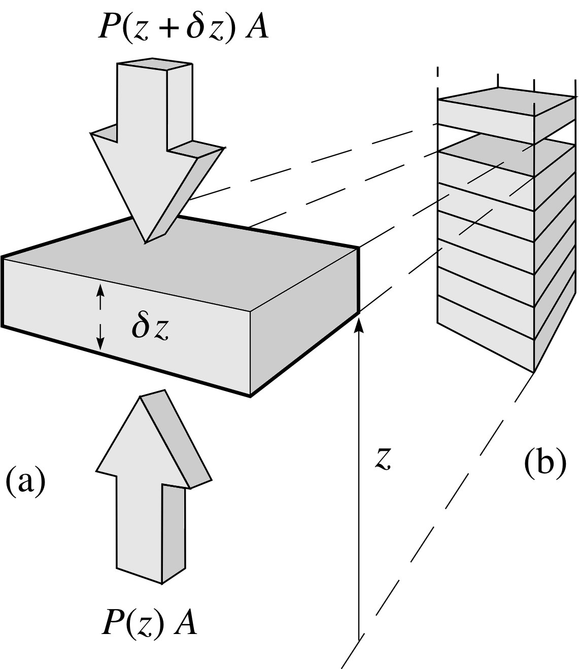
Figure 1 (a) A shallow box of air of depth δz and cross–sectional area A. The forces on the upper and lower faces are P (z + δz) A (downwards) and P (z) A (upwards). (b) A stack of such boxes.
This example introduces an important method of formulating differential equations in order to model the way in which atmospheric pressure P falls with increasing altitude z. i
We will assume that the atmosphere is everywhere in mechanical equilibrium, and we will model it as a column of air of constant cross sectional area A (see Figure 1b). We will divide this column into shallow ‘boxes’ of air, of thickness δz (you will see shortly why they must be shallow boxes i), and to construct the differential equation relating P and z, we will apply the condition for mechanical equilibrium to one of these shallow boxes (see Figure la).
As shown in Figure 1a, the pressure on the lower face of the box is P (z), while the pressure on the upper face is P (z + δz). In order that the box of air should be in equilibrium, the net upwards force due to this pressure difference must be sufficient to support the weight of the air in the box.
Since the pressure is the magnitude of the force per unit area of the box, the force due to pressure on the lower side is P (z) A, acting upwards, while the force due to pressure on the upper side is P (z + δz) A, acting downwards.
So, equating the magnitudes of the various forces:
| upward force on box | = | downward force on box | + | weight of air in box |
i.e. P (z) A = P (z + δz) A + | weight of air in box |
The magnitude of the weight of the air in the box is simply the mass of air in the box multiplied by g, the magnitude of the acceleration due to gravity. We can calculate the mass of the air in the box if we know the density of the air and the volume of the box, but here it becomes important that we have assumed that the box is very shallow. The density of the atmosphere varies with altitude; by requiring the boxes to be shallow we are justified in assuming that the density of air within any particular box is effectively constant (though the value of that ‘constant’ will vary from box to box as the altitude changes).
Thus we can say,
mass of air in box = density of air × volume of box ≈ ρ (z) Aδz(8)
where ρ (z) is the density of air at altitude z. Multiplying this mass by g gives the magnitude of the weight of the air; and so we have
P (z) A ≈ P (z + δz) A + ρ (z) Agδz i
Rearranging this equation, and dividing both sides by A, we obtain
$\dfrac{P(z + \delta z) - P(z)}{\delta z} \approx -g\rho(z)$(9)
As δz becomes smaller, the approximation we made in writing down Equation 8 becomes better and better. If we take the limit δz → 0, we can replace the approximate equality in Equation 8 and in Equation 9, by an equality. Moreover, when we do this, the quantity on the left–hand side of Equation 9 becomes (by definition) the derivative dP/dz. Thus when we take this limit, Equation 9 becomes the differential equation
$\dfrac{dP}{dz}(z) = -g\rho(z)$
This equation cannot yet be solved for P, as it contains ρ which also varies with z. To proceed further, we have to relate ρ to P.
This can be done by using the so–called equation of state of air, a simple version of which might prompt us to replace ρ (z) by aP (z), where a is a constant. This leads us to a differential equation that could be solved for P (z), though more complicated versions of the equation of state leading to more challenging differential equations are also possible.
This technique of looking at the change in the dependent variable (P) due to a small change (δz) in the independent variable (z) and then allowing this small change (δz) to tend to zero, is extremely important in mathematical modelling and you should take particular note of it. In order to reinforce this point we will now apply the technique to another case.
Water flowing from a small hole
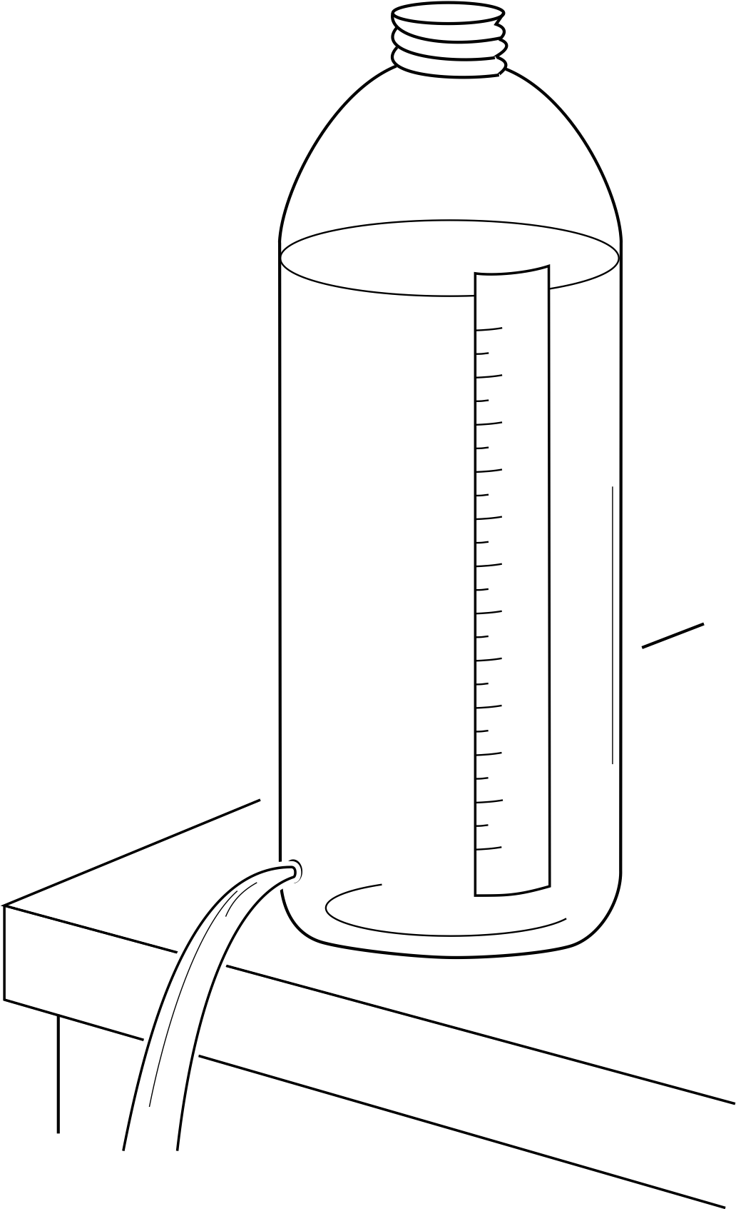
Figure 2 Water flowing from a small hole in a cylindrical bottle.
This example is concerned with the rate at which water flows out of a small hole at the bottom of a cylindrical bottle, as shown in Figure 2. The aim is to find a differential equation which determines the way in which the height y of the water level above the hole varies with time t. We do this in two steps:
- 1
-
First, we relate the rate at which the volume V of water in the bottle decreases to the speed v with which the water flows out of the hole;
- 2
-
then we find equations relating V to y and v to y, to obtain an equation that involves only one dependent variable, y, the height of the water in the bottle.
Step 1 To find an expression for the rate at which V decreases, we will consider the volume of water leaving the hole in a short time interval δt. (As in the previous example, we need to consider a short time interval so that we can assume that quantities which may vary with time, such as v, the speed of flow of the water, stay approximately constant during this time interval.)
Let the stream of water leaving the hole have a cross–sectional area a. i
If the speed of the emerging water is v at the start of the short time interval, then during time δt, a small cylinder of water of length vδt and cross–sectional area a exits from the hole. This small cylinder has volume avδt. So the change in volume V will be a negative quantity (i.e. a decrease) given by V (t + δt) − V (t) ≈ −avδt. Now, if we divide both sides of this equation by δt, we obtain
$\dfrac{V(t + \delta t) - V(t)}{\delta t} \approx -av(t)$(10)
As in the previous example, we now take the limit as δt → 0. The left–hand side of Equation 10 becomes dV/dt, and we can now replace approximate equalities by equalities. So we obtain the differential equation
$\dfrac{dV}{dt} = -av$(11)
Step 2 We now want to express V and v in terms of y. We will assume that the part of the bottle that contains water has a constant cross–sectional area A. Then V and y are simply related by V = Ay, and Equation 11 becomes
$\dfrac{d}{dt}(Ay) = -av$
and since A is a constant we can write
$\dfrac{dy}{dt} = -\dfrac aA v$(12)
We now have to relate v to y. Here, we need to bring in a law of physics that you will probably never have met before. It is called Torricelli’s theorem, and it reflects the fact that the speed v of a stream of an ideal fluid i emerging from a small hole in an open container depends on the height y of the fluid surface above the hole and is given by $v = \sqrt{2gy\os}$, where g is the magnitude of the acceleration due to gravity. This law applies to any shape of container, not just cylindrical vessels.
Using Torricelli’s theorem in Equation 12, we at last obtain a differential equation involving only y, t and constants:
$\dfrac{dy}{dt} = -\dfrac aA \sqrt{2gy\os}$(13)
Question T3
Molecules in a gas_phasegas collide with each other. Use the following information to construct a differential equation which determines the number of molecules N (x) which travel a distance x without making any collisions.
- The number of molecules N (x + δx) which travel a distance x + δx without colliding is equal to the number N (x) multiplied by the probability that a molecule does not make a collision in a distance δx.
- The probability that a molecule makes a collision in a short distance δx is approximately equal to Cδx, where C is a constant, and the approximation becomes more accurate as δx becomes smaller.
Answer T3
Since the probability that a molecule makes a collision in distance δx is approximately Cδx, the probability that it does not make a collision in this distance is approximately (1 − Cδx). We multiply this by N (x) to obtain an approximate value for N (x + δx) so that
N (x + δx) ≈ N (x)(1 − Cδx)
If we rearrange this approximate equation we get
$\dfrac{N(x + \delta x) - N(x)}{\delta x} \approx -CN(x)$
When we let δx tend to zero, the approximation becomes exact, and the quantity on the left hand–side becomes
dN/dx. So the required differential equation is
$\dfrac{dN}{dx} = -CN$
Classical mechanics
You have now seen two ways of using a differential equation to model a physics problem. You can either:
- 1
-
look out for phrases such as ‘rate of change’, ‘decay rate’, etc. and express these quantities as derivatives; i or
- 2
-
relate a small change in the dependent variable to a small change in the independent variable, and take limits as both quantities tend to zero. i
However, there is also a whole class of problems in physics which express themselves almost automatically in the language of differential equations. We have in mind problems in classical mechanics. The basic equation of classical mechanics is Newton’s second law, F = ma, i where F is the total force acting on the object of mass m and a is the acceleration of the object. However, acceleration (a) is simply the rate of change of velocity (v), so that a = dv/dt; and velocity (v) is the rate of change of position (dr/dt). So you can see that differential equations are inevitably going to arise whenever you write down the equation of motion that determines the position of an object as a function of time.
To keep things simple, we will only consider motion along a straight line, which we will take to be the x-axis of a Cartesian coordinate system. We will also restrict our considerations to objects of constant mass m. (Examples might be: a car moving along a straight road, an object dropped from a height, or a mass oscillating up and down on a spring.)
In such cases, Newton’s second law enables us to relate the x–components of force and acceleration, so we can write Fx = max. This may be rewritten as a differential equation in either of two ways (depending on what we want to know about the object’s motion):
$F_x = m\dfrac{dv_x}{dt}$(14)
or$F_x = m\dfrac{d^2x}{dt^2}$(15)
where x specifies the position of the object (i.e. its displacement from the origin), vx its velocity, and Fx the force acting on it (all these quantities are positive if directed along the positive x–axis). The force Fx here might be given as a function of time t, or as a function of position, x. It might even depend on the velocity of the object (air resistance is a force of this sort), in which case the left–hand side of Equation 15 might involve dx/dt. And, of course, there might be more than one force acting, so Fx might well be the sum of several different terms.
Once you have found expressions for all the forces acting on the object, it becomes very easy to write down the differential equation giving x (t); the only tricky part may be getting the signs of the various contributions to Fx correct. Here are some key words and phrases to look out for in similar problems:
- A ‘force acting towards the origin’ should be given a negative sign, because x is measured away from the origin.
- A ‘restoring force’ is one which tends to pull the object back to its starting point, so that if the object starts from x = 0, the direction of the force is opposite to the direction of the object’s displacement.
- A ‘resistive force’ is one where the direction of the force is always opposite to the direction of the object’s velocity.
- The words ‘repulsive’ and ‘attractive’ also give information about the direction of the force; a ‘repulsive force’ tends to increase the distance between the moving object and whatever is producing the force, while an ‘attractive force’ tends to reduce the distance.
For example, consider the following case: A moving object with position coordinate x experiences a restoring force proportional to x, as well as a resistive force proportional to its velocity. This tells us that Fx is the sum of two terms. The first is equal to −kx, where k is a positive constant. The second term is equal to −Cdx/dt, where C is another positive constant. So, in this particular case, Equation 15 becomes
$m\dfrac{d^2x}{dt^2} = -kx - C\dfrac{dx}{dt}$(16)
✦ How did we know that both these forces should have a minus sign?
✧ Because the first is a restoring force, which must have the opposite sign to x, while the second is a resistive force, which must be positive if dx/dt is negative and vice versa.
Now that you have seen some of the ways in which differential equations may arise in physics, we will spend most of the rest of this module describing the purely mathematical properties of differential equations.
3 Classifying differential equations
The next three subsections introduce some terminology that is used to classify differential equations. Familiarity with this terminology will be useful to you when you come to solve differential equations, since you will need to know what sort of differential equation you are dealing with if you want to seek advice from a mathematics textbook.
3.1 Order and degree of differential equations
Order
The order of a differential equation is the order of the highest derivative that appears in it.
Thus a first-order differential equation is one that contains the first derivative of the dependent variable, and no higher derivatives; a second-order equation contains the second derivative, and maybe the first derivative as well, but no higher derivatives; and so on. Here are some examples of differential equations of various orders:
a first-order differential equation
$y\dfrac{dy}{dx} = x$(17)
a second-order differential equation
$\dfrac{d^2y}{dx^2} + \left(\dfrac{dy}{dx}\right)^2 + x = 0$(18)
a fourth-order differential equation
$\dfrac{d^4y}{dx^4} + 3\dfrac{dy}{dx} = 0$(19)
Question T4
State the order of Equations 4, 7 and 16:
$\dfrac{dN}{dt}(t) = -\lambda N(t)\,dt$(Eqn 4)
$\dfrac{dn}{dt}(t) = kn(t)[N_0 - n(t)]$(Eqn 7)
$m\dfrac{d^2x}{dt^2} = -kx - C\dfrac{dx}{dt}$(Eqn 16)
Answer T4
Equation 4,
$\dfrac{dN}{dt}(t) = -\lambda N(t)\,dt$(Eqn 4)
is first order; only the first derivative of the dependent variable appears. Similarly Equation 7,
$\dfrac{dn}{dt}(t) = kn(t)[N_0 - n(t)]$(Eqn 7)
is first order. In Equation 16,
$m\dfrac{d^2x}{dt^2} = -kx - C\dfrac{dx}{dt}$(Eqn 16)
the highest order derivative appearing is the second derivative of x; therefore it is second order.
Degree
The degree of a differential equation is the highest power to which the highest order derivative in the equation is raised.
Thus Equations 17–19 are all of the first degree; in each case, the highest derivative present is raised to the first power. (Although the square of dy/dx appears in Equation 18, this is irrelevant when establishing the degree of the equation because dy/dx is not the highest order derivative present in the equation.)
Here are two equations of degree higher than the first:
a second–degree differential equation
$\left(\dfrac{dy}{dx}\right)^2 + \dfrac{dy}{dx} + y = 0$
a third–degree differential equation
$\left(\dfrac{d^2y}{dx^2}\right)^3 + \dfrac{dy}{dx} + x = 0$
The definition we have given of the degree of a differential equation only applies if all derivatives in the equation are raised to integer (i.e. whole number) powers. If this is not the case, we must carry out the process of rationalization before deciding on its degree, that is, we must manipulate the equation so that all fractional powers of derivatives are removed. For example, consider the equation
$\dfrac{d^2y}{dx^2} = \sqrt{\dfrac{dy}{dx}}$
To identify its degree, we must square both sides of the equation, to obtain
$\left(\dfrac{d^2y}{dx^2}\right)^2 = \dfrac{dy}{dx}$
and we see that it is of second degree.
Question T5
What are the degrees of the two following differential equations?
(a) $\left(\dfrac{dy}{dx}\right)^2\dfrac{d^2}{dx^2} + y^3 = 0$
(b) $x\left(\dfrac{dy}{dx}\right)^2 + \sqrt{y\os} = \dfrac{dy}{dx}$
Answer T5
(a) In this equation, the highest derivative present is d2y/dx2, and it is raised to the first power. The equation is therefore of first degree.
(b) In this equation, the highest derivative present is dy/dx, and it is raised to the power 2. The equation is therefore of second degree. Note that in this case there is no need to rationalize the power of y appearing in the equation. It is only when derivatives of the dependent variable appear raised to fractional powers that the equation needs to be rationalized.
3.2 Linear differential equations
This is the full mathematical definition of a linear differential equation. (It looks worse than it really is.)
A linear differential equation of order n is an equation of the form
$a(x)\dfrac{d^ny}{dx^n} + b(x)\dfrac{d^{n-1}y}{dx^{n-1}} + \cdots + g(x)\dfrac{dy}{dx} + r(x)y = f(x)$(20)
where the coefficients a (x), b (x), etc. on the left–hand side and the function f (x) on the right–hand side are arbitrary functions of x (which includes the possibility that some of them may be constants, or zero).
We can characterize a linear differential equation by saying that it must have the following properties:
- 1
-
The dependent variable y and its derivatives must appear raised only to the first power. Thus there can be no terms like (dy/dx)2 or $\sqrt{y\os}$.
- 2
-
Functions of y or of its derivatives such as ey or tan(dy/dx) are forbidden, as are terms like 1/(y + x).
- 3
-
The equation must not contain products of derivatives of different order, or of y with its derivatives. Thus there can be no terms like $y\dfrac{dy}{dx}$ or $\dfrac{dy}{dx}\dfrac{d^2y}{dx^2}$.
Note that an equation that can be written in the form shown in Equation 20 (i.e. possessing properties 1, 2 and 3) simply by moving terms from one side of the equation to the other is also considered to be linear. (For example, $\dfrac{dy}{dx} = -x^3y + \sin x$ and $\dfrac{1}{dy/dx} = \dfrac1y$ are both linear as they can be written as $\dfrac{dy}{dx} + x^3y = \sin x$ and $\dfrac{dy}{dx} - y = 0$, respectively.)
Notice in particular that the independent variable x is allowed to appear in any form whatsoever in a linear differential equation. The functions of x appearing on the right–hand side of Equation 20, or as coefficients of y and its derivatives, may be extremely complicated but the equation will still be linear.
✦ What is the degree of a linear differential equation?
✧ A linear differential equation only contains derivatives raised to the first power. So by definition, the derivative of highest order present must be raised to the first power. All linear differential equations are therefore of the first degree.
The examples that follow should help to make the idea of a linear differential equation clear.
Example 1
Is the equation $\dfrac{d^2y}{dx^2} - \tan y = 0$ linear?
Solution
No, it is not linear, because of the presence of the term tan y.
Example 2
Is the equation $\dfrac{d^2y}{dx^2} + y\dfrac{dy}{dx} + xy = 0$ linear?
Solution
No, it is not linear, because of the presence of the product $y\dfrac{dy}{dx}$.
Example 3
Is the equation $x^2\dfrac{d^2y}{dx^2} + x\dfrac{dy}{dx} - \loge x = y$ linear?
Solution
Yes. We may rewrite it in the form of Equation 20,
$a(x)\dfrac{d^ny}{dx^n} + b(x)\dfrac{d^{n-1}y}{dx^{n-1}} + \cdots + g(x)\dfrac{dy}{dx} + r(x)y = f(x)$(Eqn 20)
as$x^2\dfrac{d^2y}{dx^2} + x\dfrac{dy}{dx} - y = \loge x$
Instead of comparing it with Equation 20, we may equally well argue that as y and its derivatives only appear raised to the first power, and as there are no products among y and its derivative, and no functions of y, the equation is linear.
Study comment In answering the following question, you should ask yourself whether the equation satisfies the three properties given above, or, if this does not decide the matter, try to rewrite the equation in the form of Equation 20. Eventually, you will probably be able to see at a glance whether or not a given differential equation is linear, but this takes some practice.
Question T6
Explain whether or not Equations 4, 7, 13, 16 and 17 are linear:
$\dfrac{dN}{dt}(t) = -\lambda N(t)\,dt$(Eqn 4)
$\dfrac{dn}{dt}(t) = kn(t)[N_0 - n(t)]$(Eqn 7)
$\dfrac{dy}{dt} = -\dfrac aA \sqrt{2gy\os}$(Eqn 13)
$m\dfrac{d^2x}{dt^2} = -kx - C\dfrac{dx}{dt}$(Eqn 16)
$y\dfrac{dy}{dx} = x$(Eqn 17)
Answer T6
Equations 4 and 16,
$\dfrac{dN}{dt}(t) = -\lambda N(t)\,dt$(Eqn 4)
$m\dfrac{d^2x}{dt^2} = -kx - C\dfrac{dx}{dt}$(Eqn 16)
are linear; the dependent variables and their derivatives appear raised only to the first power, and there are no products or functions of the dependent variables or their derivatives with one another in either equation.
Equation 7,
$\dfrac{dn}{dt}(t) = kn(t)[N_0 - n(t)]$(Eqn 7)
is not linear; there is a term containing the square of the dependent variable on the right–hand side.
Equation 13,
$\dfrac{dy}{dt} = -\dfrac aA \sqrt{2gy\os}$(13)
is not linear; the square root of the dependent variable appears on the right–hand side.
Equation 17,
$y\dfrac{dy}{dx} = x$(17)
is not linear, due to the presence of the product of the dependent variable and its first derivative.
3.3 Non–linear differential equations
What about differential equations that are not linear? They are simply called non–linear differential equations. This terminology rather suggests that linear differential equations are very much more important than non–linear ones. There are two arguments that might be used to support this view. First, most differential equations that we encounter in physics are linear. Second, linear differential equations are much easier to solve than non–linear ones.
However, neither of these arguments stands up to close scrutiny. It is true that many of the fundamental differential equations of physics – such as Schrödinger’s equation (the basic equation of quantum mechanics) or maxwells_theory_of_electromagnetismMaxwell’s equations describing the behaviour of electric_fieldelectric and magnetic fields in a vacuum are linear. But some are not; for example, the equations describing gravitational phenomena in Einstein’s einsteins_special_theory_of_relativitygeneral theory of relativity. As soon as you start to apply laws of physics to large scale phenomena you are very likely to run into a non-linear differential equation. Until recently, the expected response would have been to turn your non–linear equation into a linear one by making suitable approximations. Here is an example of this procedure which is known as linearization.
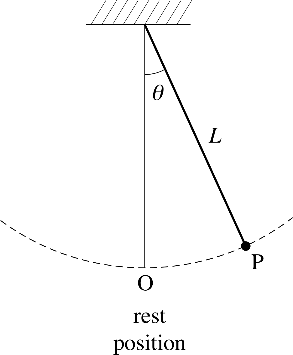
Figure 3 A simple pendulum consisting of a weight (the bob at P) which is suspended from a fixed position by a light rod or string of length L, and moves in an arc through its rest position O.
A simple pendulum (see Figure 3) moving in a plane, has an equation of motion (which we will not derive) as follows:
$\dfrac{d^2\theta}{dt^2} = -\dfrac gL \sin\theta$(21) i
This is a non–linear equation (because of the presence of the sin θ term). It does not have a solution for θ in terms of ‘elementary’ functions of t (e.g. sin, cos, exp, log), though its solution can be expressed in terms of functions known as elliptic functions, which have been extensively investigated. However, if we are only concerned with small oscillations of the pendulum, for which θ ≪ 1 radian (meaning θ is very much smaller than 1 radian), we may use the approximation sin θ ≈ θ on the right–hand side, to obtain
$\dfrac{d^2\theta}{dt^2} = -\dfrac gL \theta$(22)
which is a linear equation, and can be solved very easily.
If we really are only interested in small–amplitude oscillations, then of course Equation 22 may be quite adequate as an approximation to Equation 21, but the real trouble with Equation 22 is that there are important qualitative features of the motion of the pendulum that it gets entirely wrong. For example, the pendulum shown in Figure 3 clearly has a position of unstable equilibrium where the bob is at rest at a point diametrically opposite to the position of stable equilibrium (at O), and this corresponds to θ = π and $\dfrac{d^2\theta}{dt^2} = 0$ i This is a solution of Equation 21 (since sin π = 0), but is clearly not a solution of Equation 22. Similarly, although we will not prove this, Equation 21 possesses solutions where θ always increases with time – the pendulum bob swings round and round in a circle in a plane – which are not solutions of Equation 22.
In other words, by linearizing Equation 21, we have thrown away the possibility of ever discovering a number of interesting features of the behaviour of the pendulum. In the present case, this is not a disaster, since we have a good knowledge of the way in which a pendulum can behave. But when a non–linear differential equation is used to describe less well–understood phenomena, there is a real danger that by linearizing it we would lose much valuable information.
This brings us back to the other point mentioned above – that linear differential equations are easier to solve. It is certainly true that there exist methods of solving linear equations that cannot be applied to non–linear ones. However, when it comes to investigating the qualitative features of a system’s behaviour, there are approaches that can as readily be applied to non–linear equations as to linear ones (although we will not discuss them here). Non–linear differential equations are a subject of current research for many physicists and applied mathematicians.
4 Solving differential equations (generalities)
4.1 What is a solution of a differential equation?
When we solve an algebraic equation (such as x2 − 5x + 6 = 0), our aim is to find the unknown number or numbers x that satisfy the equation. By contrast, when we solve a differential equation, we want to find the unknown function or functions that satisfy the equation. To put this more precisely:
A solution to a differential equation is a relation between the variables y and x in which no derivatives appear, and which is such that if we substitute it into the original equation we find that equation becomes an identity. i
For example, consider the differential equation
$\dfrac{dy}{dx} = x$(23)
We claim that y = x2/2 is a solution of this equation. To see whether or not this is so, we substitute y = x2/2 into the equation. The first derivative of x2/2 is equal to x, and so on making this substitution the equation becomes x = x, which is indeed an identity. Thus y = x2/2 is a solution of the differential equation; alternatively, we say that y = x2/2 satisfies the equation.
Systematic methods of finding solutions of different types of equations are considered elsewhere in FLAP. However, if you have reason to believe that a certain relation between y and x will solve the differential equation, then all you need to do is to substitute the relation into the original equation. If this gives you an identity then the relation is indeed a solution; otherwise, it is not.
Example 4
Show that the differential equation $x^2\dfrac{d^2y}{dx^2} = 2y$ has a solution of the form y = x n, and find the value or values of the exponent n.
Solution
Differentiating y = x n once gives dy/dx = n x n−1; differentiating dy/dx to obtain the second derivative gives
$\dfrac{d^2y}{dx^2} = n(n-1)x^{n-2}$
On substituting y and its second derivative into the original differential equation, we obtain
x2[n (n − 1) x n−2] = 2x n
i.e.n (n − 1) x n = 2x n
which is an identity provided that n (n − 1) = 2. This quadratic equation for n is satisfied if n = 2 or if n = − 1. So the equation does possess solutions of the given form; they are y = x2 and y = 1/x.
Question T7
Show by substitution that y = e−x is a solution of the differential equation $\dfrac{dy}{dx} = -y$
Answer T7
If y = e−x, then dy/dx = −e−x. Thus substituting y and its derivative into the differential equation gives us −e−x = −e−x, which is an identity. So y = e−x is a solution.
The solutions to Equation 23 and to the equations given in Example 4 and Question T7 could all be written in the form y = f (x). This will normally be true for the differential equations you encounter in physics. However, it is possible for a differential equation to lead to a relation between x and y where we cannot make y the subject of the equation (in other words, we cannot rearrange the equation into the form ‘y = some function of x’). For example, we might find that a certain differential equation was satisfied if y and x were related by the equation
$y + \loge{y} = x^3 + x$(24)
You will find that, however hard you try, you will not be able to manipulate Equation 24 so as to put it into the form ‘y = function of x’. However, for any given value of x, we could, with sufficient time and ingenuity, calculate the corresponding value of y. Thus Equation 24 does define y as a function of x, though it does not do so explicitly. We say that it gives y as an implicit function of x.
4.2 General solutions and particular solutions
We showed in Subsection 4.1 that y = x2/2 was a solution of Equation 23,
$\dfrac{dy}{dx} = x$(Eqn 23)
however, it is not the only solution. Suppose we try substituting into Equation 23 the relation y = (x2/2) + C, where C is an arbitrary constant. Since the first derivative of $\left(\dfrac{x^2}{2} + C\right)$ is also equal to x, then $y = \dfrac{x^2}{2} + C$ is a solution of the equation for any value of the constant C. We say that it is a general solution of the equation, meaning that it involves an arbitrary constant, and that for any choice of that arbitrary constant, it is a solution of the differential equation. You can see that it gives us a whole ‘family’ of solutions, one for each of the (infinite number of) values of the constant C.
A specific choice for the arbitrary constant C gives us what is called a particular solution of the differential equation – a solution which does not contain any arbitrary constants. The solution we found originally, y = x2/2, is a particular solution of Equation 23, corresponding to C = 0.
Question T8
Show by substitution that y = C e−x is a solution of the differential equation dy/dx = −y, where C is an arbitrary constant.
Answer T8
If y = C e−x, then dy/dx = −C e−x. Thus substituting y and its derivative into the differential equation gives us −C e−x = −C e−x, which is an identity. So y = C e−x is a general solution.
We have seen that Equation 23,
$\dfrac{dy}{dx} = x$(Eqn 23)
possesses an infinite number of solutions, all of the form $y = \dfrac{x^2}{2} + C$. Are there any other solutions? It is easy to show that there are no other solutions by solving Equation 23 in another way. The differential equation states that the derivative of y with respect to x is equal to x; in other words, y is the inverse derivative (i.e. the indefinite integral) of x. But this indefinite integral is well known, it’s just $y = \dfrac{x^2}{2} + \text{constant }(C)$. The family of functions $y = \dfrac{x^2}{2} + C$ therefore contains all the solutions to Equation 23. We say that it is not only a general solution, but the most general solution, meaning that there is no solution to the differential equation that does not belong to this family.
The method we have just used to find the most general solution to Equation 23 is called the direct integration method for solving differential equations. It can be applied to any differential equation of the form
$\dfrac{dy}{dx} = f(x)$(25)
since any such equation states that y is the inverse derivative of f (x). Thus if we have found some function F (x) such that dF/dx = f (x), all solutions to Equation 25 are of the form y = F (x) + C. We can take this argument further. Suppose that instead of the first–order Equation 25, we wish to solve the second–order equation $\dfrac{d^2y}{dx^2} = f(x)$, then we can rewrite this equation as $\dfrac{d}{dx}\left(\dfrac{dy}{dx}\right) = f(x)$ and perform the indefinite integral, which this time gives us dy/dx rather than y, to obtain dy/dx = F (x) + C.
Now we can integrate a second time, to find y itself. This introduces a second arbitrary constant, so we obtain y (x) = G (x) + Cx + D, where G (x) is any function such that dG/dx = F (x). Again we have found a family of solutions, the members of which differ from each other only in the different values of the arbitrary constants C and D. Here we have two arbitrary constants, rather than one as in the general solution to Equation 25. Note that since we have found y by integrating directly, we can be quite sure that there are no further solutions to this equation; thus we have found the most general solution.
It is not difficult to show that the most general solution of a differential equation of the form
$\dfrac{d^ny}{dx^n} = f(x)$(26)
will contain n arbitrary constants, and, more generally, it can be proved that:
Any linear differential equation of order n possesses a general solution containing n independent arbitrary constants, and all particular solutions to such an equation can be obtained by choosing particular values for these constants.
Note that the arbitrary constants appearing in the general solution must be independent. Two (or more) arbitrary constants are said to be independent if they cannot be combined into one constant. For example, the two arbitrary constants A and B in the following equation are not independent:
y = Ax + Bx + x2
because (Ax + Bx) can be written as Cx, where C is another (arbitrary) constant, giving y = Cx + x2
On the other hand, the constants A and B in y = A + Bx + x2 are independent, because A and B cannot be combined; one multiplies the variable x, the other does not. Independent arbitrary constants are often called essential constants.
Considerations such as these are important if you want to see whether or not a solution you think you have found to a given differential equation is a general solution. There are two steps involved in checking this:
- 1
-
You should obviously make sure that it is a solution, i.e. that it satisfies the original equation.
- 2
-
If it is a solution, you should count the number of independent arbitrary constants it contains. If the differential equation is of order n, then a solution to it must contain n essential constants (independent arbitrary constants) to be a general solution.
Example 5
If A and B are arbitrary constants, show that
y = A sin x + B cos x(27)
is a general solution of
$\dfrac{d^2y}{dx^2} + y = 0$(28)
Solution
First check to see whether Equation 27 is a solution. Differentiating y once gives
dy/dx = A cos x − B sin x
Differentiating again to find d2y/dx2 gives
$\dfrac{d^2y}{dx^2} = -A\sin x - B\cos x = -y$ (from Equation 27)
Thus Equation 27 is a solution to Equation 28. This solution contains two arbitrary constants, which multiply different functions of x, and so are independent. As Equation 28 is of second order, its general solution should contain two essential constants. So Equation 27 does indeed give the general solution of Equation 28.
Question T9
Consider the linear differential equation
$\dfrac{d^2y}{dx^2} - 3\dfrac{dy}{dx} + 2y = 0$
Is y = A e(x+B), where A and B are arbitrary constants, a solution of this equation? Is it a general solution?
Answer T9
To see whether y = A e(x+B) is a solution, we substitute it into the equation. Note that we can write this function as A exeB, and that A eB is simply a constant; so we have
$\dfrac{dy}{dx} = A{\rm e}^B{\rm e}^x\quad\text{and}\quad\dfrac{d^2y}{dx^2} = A{\rm e}^B{\rm e}^x$
On substitution, we find that the left–hand side of the equation in Question T9 becomes
A eBex − 3A eBex + 2A eBex
which is identically equal to zero. Thus we have a solution. But we have seen that we can write this solution as y = A eBex, where A eB is a constant that we may call C. Thus the two constants appearing here are not independent; the solution can be written as y = C ex, showing explicitly that it contains only one essential constant. It therefore cannot be the general solution to this second–order equation, which must contain two essential constants.
Solving non–linear differential equations
We end this subsection with some remarks on non–linear differential equations and their solutions. First, although it is generally true that a non–linear differential equation of order n possesses a general solution containing n essential constants, the solutions may involve complex numbers. i
Second, non–linear differential equations often possess particular solutions which cannot be obtained from the general solution by assigning certain values to the arbitrary constants. These solutions are called singular solutions.
For example, consider the non–linear first–order differential equation
$\dfrac{dy}{dx} = 2\sqrt{y-1\os}$(29)
We can show by substitution that this equation has a general solution
y = 1 + (x + C)2(30)
where C is an arbitrary constant. If we differentiate y we find
$\dfrac{dy}{dx} = 2(x + C)$(31)
and, from Equation 30, x + C = y − 1, so Equation 30 is satisfied. But Equation 29 can also be satisfied by the very simple solution y = 1. We cannot obtain this from the family of solutions given by Equation 30 for any choice of the constant C. So, while Equation 30 gives a general solution, it does not contain all possible solutions. In a physics problem described by a non–linear differential equation, it is usually the general solution that is relevant. However, singular solutions do sometimes have physical significance.
4.3 Initial conditions and boundary conditions
Suppose you have managed to find a general solution y = f (x) to a differential equation that has arisen in some problem in physics. Since this solution (by definition) contains one or more arbitrary constants, you have not yet managed to determine y uniquely as a function of x. But a specific problem in physics normally requires a unique answer – a particular solution, in other words. Evidently you will require more information than is provided by the differential equation alone in order to assign appropriate values to the arbitrary constants and so obtain the appropriate particular solution.
To see what sort of information is necessary, let us return to the example of radioactive decay introduced in Subsection 2.2. We showed there that the differential equation that determined the number N of radioactive atoms present at time t is
$\dfrac{dN}{dt}(t) = -\lambda N(t)$(Eqn 4)
where λ is the decay constant of the radioactive substance. A general solution to this equation is
N = A e−λt, where A is an arbitrary constant
✦ Check that this is a general solution of Equation 4.
✧ It is a solution because
$\dfrac{d}{dt}(A{\rm e}^{-\lambda t}) = -\lambda A{\rm e}^{-\lambda t}= -\lambda N$
It is a general solution to the first–order Equation 4 because it contains one arbitrary constant, A. (The decay constant λ is not an arbitrary constant, it is a parameter of the problem and so has a definite value.)
If we want to calculate actual values for N at different times t, the general solution is of no use, as it contains the unknown constant A. But we can find a value for A if we are told the value of N at some particular time t0. If N has the value 1020 at that time, then we can determine A from the relation
1020 = A e−λt0
Clearly the most convenient value for t0 would be t0 = 0, as then we have simply A = 1020. Indeed we usually (though not always) decide to define t = 0 as the time at which the extra information we need to determine the arbitrary constants is specified. If we do that here, the particular solution is
N (t) = 1020e−λt
from which (assuming we know the value of λ) we can calculate the value of N at any later time t.
A condition of the sort ‘N = 1020 at t = 0’, providing us with the extra data we need to determine the values of the arbitrary constants in the general solution, is called an initial condition. In the case we have just discussed, we needed one initial condition to find the value of the one arbitrary constant that appeared in the general solution to a first–order differential equation. The differential equation in the following question is of second order, so you will need two initial conditions to find the values of the two arbitrary constants.
Question T10
An object’s position coordinate x satisfies a differential equation which has the general solution x = A cos ωt + B sin ωt, where ω is a constant. Find values for the arbitrary constants A and B if at t = 0, the object is located at x = 0.01 m and its velocity is zero.
Answer T10
We first substitute the values t = 0, x = 0.01 m into the expression for x, which gives 0.01 m = A cos + B sin 0, i.e. A = 0.01 m. Differentiating x to find the velocity as a function of time t gives us dx/dt = −A sin t + B cos t, and substituting the values t = 0, dx/dt = 0 gives us 0 = −A sin 0 + B cos , i.e. B = 0. Thus the values of the constants are A = 0.01 m, B = 0.
In this question we needed the values of x and vx at t = 0 in order to find the constants A and B. Could we not instead have specified the value of x at two different times? That would surely have led to two equations which could be solved for A and B. The answer is that, while in the present case that would have worked, it does not always do so! Consider the following example (apparently, but deceptively, very similar to Question T10).
Example 6
An object’s displacement x satisfies a differential equation which has the general solution x = A cos ωt + B sin ωt. Find values for the arbitrary constants A and B if x = 0 at t = 0 and also x = 0 at t = π/ω.
Solution
If we apply the first condition we find 0 = A cos 0 + B sin 0; and since cos 0 = 1 while sin 0 = 0, we conclude that A = 0. However, if we apply the second condition, we obtain 0 = A cos π + B sin π and since cos π = −1 and sin π = 0, we simply find A = 0 again! In this case, although we have two specific pieces of information about the object’s displacement, they are not sufficient to allow us to determine the values of both the arbitrary constants A and B.
In contrast, for the general linear differential equation of order n (given by Equation 20)
$a(x)\dfrac{d^ny}{dx^n} + b(x)\dfrac{d^{n-1}y}{dx^{n-1}} + \cdots + g(x)\dfrac{dy}{dx} + r(x)y = f(x)$(Eqn 20)
it can be proved that the values of y, dy/dx, d2y/dx2 and all derivatives up to d n−1y/dx n−1 at a particular value of x, are sufficient to determine unique values for the n essential constants. This result is called a uniqueness theorem.
The equations specifying the value of y and of as many of its derivatives as are necessary at some chosen value of x are usually called initial conditions, even when the independent variable is not time! If, instead, we are given information about y and/or its derivatives at different values of the independent variable, the equations giving this information are called boundary conditions. You have seen an example where n boundary conditions are not sufficient to determine n arbitrary constants. Very often, however, they do provide enough information to evaluate the arbitrary constants.
Finally, you will have noticed that the uniqueness theorem applies specifically to linear differential equations. What about non–linear ones? While it is possible to prove that, under certain conditions, n initial conditions are necessary and sufficient to determine a unique particular solution to a non–linear differential equation of order n, the conditions that need to be stated are rather complicated, and we will not go into them here. You will find that for most of the non–linear differential equations you encounter in physics, the given initial conditions determine a unique solution, however, you should always bear in mind the possibility that they may not.
4.4 The future from the past: determinism and chaos
You have now seen that the use of differential equations in physics involves three steps:
- 1
-
We first need to set up a differential equation to describe the system in which we are interested.
- 2
-
We must then obtain the general solution to the differential equation.
- 3
-
Finally, we apply initial (or boundary) conditions to obtain the appropriate particular solution.
Step 3 does not always lead to a unique particular solution. However, in this subsection, we will only be concerned with the (very common) situation where initial conditions do determine a unique particular solution. In such a case, once we are given the differential equation and the initial conditions, we can calculate the value of the dependent variable for any given value of the independent variable.
Motion under gravity
Consider, for example, the motion of a ball thrown vertically up into the air so that it experiences a constant downward acceleration due to gravity. If its position coordinate (measured vertically upwards from some arbitrarily chosen origin) is x at time t then
$\dfrac{d^2x}{dt^2} = -g$(32)
where g is the magnitude of the acceleration due to gravity. If the initial conditions are x = x0 and dx/dt = ux when t = 0, i then the particular solution of this differential equation is
$x = -\dfrac{gt^2}{2} + u_xt + x_0$(33)
(You could check that this is so by first differentiating twice to show that this is a solution, then by showing that the initial conditions are satisfied.)
Question T11
In the motion of a ball, given that x0 = 1 m and ux = 15 m s−1, and assuming that g = 10 m s−2, what are the displacement and velocity at t = 2 s? At what time does it return to its starting point (i.e. x = 1 m), and what is its velocity vx at this point?
Answer T11
With g = l0 m s−1 Equation 33,
$x = -\dfrac{gt^2}{2} + u_xt + x_0$(Eqn 33)
gives
x = −(5 m s ) t2 + (15 m s−1) t + 1 m
andvx = dx/dt = −(10 m s−1) t + 15 m s−2
Substituting t = 2 s into these equations, we find x = 11 m, vx = −5 m s−1. When the ball returns to its starting point, x = 1 m. Thus −(5 m s ) t + (15 m s ) t = 0. This equation is satisfied by t = 0 or by t = 3 s. So the ball returns to its starting point at t = 3 s. Its velocity at this point is −15 m s−1.
In the case where the independent variable is time t, we may say that the differential equation allows us to predict the future behaviour of the system from its past behaviour (as specified by the initial conditions). A system like this, where knowledge of the differential equation governing the system and of the initial conditions allows the subsequent behaviour of the system to be predicted exactly, is called a deterministic system.
Many classical physicists and mathematicians believed that the entire Universe was a deterministic system. Let us imagine writing down the equations of motion determining the positions of every single particle in the Universe. This would be an impossibly complicated task in practice, of course; but we know that these equations would be second–order differential equations since they would all come ultimately from Newton’s second law, which is a second–order differential equation. Thus to obtain a unique solution to this set of equations, we would need two initial conditions for each particle, their positions and velocities at some initial time. Given these, all the subsequent motions of the particles would be uniquely determined, and, in the words of the 18th-century mathematician Pierre Simon de Laplace (1749–1827), ‘nothing could be uncertain, and the future just like the past would be present before [our] eyes’.
However, before concluding that everything can in principle be predicted exactly, we ought to consider how we actually obtain the initial conditions that we use to determine the unique solution to a differential equation. These must be obtained by measurement, and all measurements are subject to some experimental uncertainty, which will lead to uncertainty in the solution and the predictions that we use it to make. But does this really matter? A small uncertainty in the initial conditions will presumably only lead to a small uncertainty in our predictions; and presumably we can also imagine making the uncertainty ‘as small as we like’.
Question T12
Consider again the ball thrown up into the air. Suppose now that its initial velocity is 15.015 m s−1, and its initial displacement 1.00 m, so that its displacement is now given as a function of time by
$x = -\frac12gt^2 + 15.015 t + 1.001$
We have made a change of 0.1% in our initial conditions. Calculate the displacement and velocity of the ball at t = 2.000 s, and the time at which it returns to its starting point, working to three significant figures. Express the difference between these answers and the corresponding answers obtained in Question T11 as percentages. Again, assume that g is exactly 10 m s−2.
Answer T12
With g = l0 m s−2, we have
x = −(5.000 m s−2) t2 + (15.015 m s−1) t + 1.001 m
andvx = dx/dt = −(l0.000 m s−2) t + 15.015 m s−1
Substituting t = 2 s into these equations, we obtain x = 11.031 m, vx = −4.985 m s−1. These differ from the results obtained in Question T12 by 0.3%.
When the ball returns to its starting point, x = 1.001 m. Thus −(5.000 m s−2) t + (15.015 m s−1) t = 0.
This equation is satisfied by t = 0 or by t = 3.003 s. So the ball returns to its starting point at t = 3.003 s, which differs from the answer obtained in Question T11 by 0.1%.
The answer to Question T12 shows that in this case, a small change in initial conditions leads only to a small difference in the subsequent behaviour. However, this is not always true. It is true if the differential equation in question is linear (as is the equation of motion of the ball). It is not necessarily true if the equation is non-linear. Systems described by non–linear differential equations may be extremely sensitive to small changes or uncertainties in the initial conditions, and two systems described by the same non–linear equation but with slightly different initial states may behave completely differently at subsequent times. Such systems are said to exhibit the property of chaos.
A system displaying chaotic behaviour cannot be completely predictable, since any uncertainty – even one ‘as small as we like’ – in the initial conditions will rapidly be amplified as time goes on, thus even though the system is deterministic, in the sense described above, this is of little use to us in predicting its subsequent development since we can never know the initial conditions with infinite precision.
The Universe contains some surprises for us after all.
5 Closing items
5.1 Module summary
- 1
-
Equations involving the derivatives of functions are known as differential equations, and such equations arise in a variety of circumstances in physics.
- 2
-
A solution of a differential equation is a relation between the dependent variable, y say, and the independent variable, x say, in which no derivatives appear, and which is such that if we substitute it into the original equation we find that equation becomes an identity.
- 3
-
The Subsection 3.1order of a differential equation is the order of the highest derivative in the equation. The Subsection 3.1degree of a differential equation is the highest power to which the highest order derivative in the equation is raised. For example, the differential equation $\left(\dfrac{d^2y}{dx^2}\right)^3 + \dfrac{d^4y}{dx^4} = 0$ is of order four and degree one.
- 4
-
The general solution of a differential equation of order k (commonly) involves k arbitrary (essential) constants.
- 5
-
A particular solution is a solution that contains no arbitrary constants.
- 6
-
Initial conditions (usually conditions that apply when the independent variable is zero) in which the dependent function and its derivatives are given at any common value of the independent variable, may be used to determine a particular solution, and then to predict the values of the dependent variable. Boundary conditions which are given at different values of the independent variable may be used for the same purpose (but may not lead to a unique solution).
- 7
-
A linear differential equation of order n is an equation of the form
$a(x)\dfrac{d^ny}{dx^n} + b(x)\dfrac{d^{n-1}y}{dx^{n-1}} + \cdots + g(x)\dfrac{dy}{dx} + r(x)y = f(x)$(Eqn 20)
where the coefficients a (x), b (x), etc. on the left–hand side and the function f (x) on the right–hand side are arbitrary functions of x. Techniques exist for solving linear differential equations (but they are not discussed in this module).
- 8
-
A Subsection 3.3non-linear differential equation is generally difficult to solve, but may be linearized by making appropriate approximations. However, the resulting linear equation may have solutions that are qualitatively different from the solutions of the original non–linear equation.
- 9
-
Differential equations can be used to model mathematically a wide variety of different physical situations. One important technique used in formulating such models involves relating a small change in the dependent variable to a small change in the independent variable and taking limits as both quantities tend to zero.
- 10
-
The first–order differential equation dN/dt = kN is particularly important since it can be used to model many physical situations such as radioactive decay (k = −λ) and population growth (k = η).
- 11
-
The method of direct integration can be applied to any differential equation of the form dy/dx = f (x).
5.2 Achievements
Having completed this module, you should be able to:
- A1
-
Define the terms that are emboldened and flagged in the margins of the module.
- A2
-
Use information given in the statement of a simple problem in physics to derive a differential equation appropriate to that problem.
- A3
-
State the order and degree of a given differential equation.
- A4
-
Distinguish between linear and non–linear differential equations, and state whether a given differential equation is linear or non-linear.
- A5
-
Show by substitution whether or not a given function is a solution to a given differential equation.
- A6
-
Explain the difference between a general solution and a particular solution, and state whether or not a given solution to a differential equation is a general solution.
- A7
-
Use initial conditions and boundary conditions to obtain a particular solution from a general solution.
- A8
-
Use a given particular solution to a differential equation describing the time evolution of some system to predict the future behaviour of the system by calculating values of the dependent variable at later times.
Study comment You may now wish to take the following Exit test for this module which tests these Achievements. If you prefer to study the module further before taking this test then return to the topModule contents to review some of the topics.
5.3 Exit test
Study comment Having completed this module, you should be able to answer the following questions, each of which tests one or more of the Achievements.
Question E1 (A2)
A particle is travelling in a straight line through a gas. The speed of the particle at time t is v(t). As it travels, the particle loses energy (by collisions with gas molecules) and slows down until it eventually comes to rest. A number of different proposals concerning the way in which the particle slows down are listed below. In each case, obtain a differential equation describing the way in which the particle’s speed varies with time.
(a) The particle’s speed decreases at a constant rate.
(b) The deceleration of the particle at time t is proportional to t.
(c) The resistive force acting on the particle is proportional to the kinetic energy of the particle. (The kinetic energy at time t is ½ m [v (t)]2, where m is the constant mass of the particle.)
(d) The change in the particle’s speed over a short time interval δt is approximately proportional both to δt and to the speed of the particle at the start of the interval. This approximation becomes more accurate as δt becomes smaller.
(e) The speed changes in such a way that over a short time interval δt, the kinetic energy [as defined in part (c)] is reduced by an amount approximately proportional to the product of δt and the speed at the start of the interval. This approximation becomes more accurate as δt becomes smaller.
Answer E1
(a) The rate at which the particle’s speed decreases is −dv/dt, and this is equal to a constant. So the required differential equation is
$\dfrac{dv}{dt} = -k$
where k is a positive constant.
(b) The deceleration of the particle is equal to −dv/dt, and this is proportional to t. So the required differential
equation is
$-\dfrac{dv}{dt} = kt\quad\text{or}\quad\dfrac{dv}{dt} = -kt$
where k is a positive constant.
(c) Again, the rate of change of speed dv/dt must be negative since the object is slowed by a resistive force. The (positive) magnitude of this rate of change must be the same as the magnitude of the acceleration, | dvx /dt | which can be determined from the one–dimensional form of Newton’s second law. Thus
$\dfrac{dv}{dt} = -\left\vert\,\dfrac{dv_x}{dt}\,\right\vert = \dfrac{\left\vert\,-F_x\,\right\vert}{m} = \dfrac{-kmv^2/2}{m}$
where k is a positive constant.
So, the required differential equation is
$m\dfrac{dv}{dt} = -\dfrac12kmv^2$ or, if we divide by m, $\dfrac{dv}{dt} = -\dfrac12kv^2$
(d) The change in v in this time interval is v (t + δt) − v (t). This change is approximately proportional to v and to δt, and is negative (since the particle is slowing down); we may therefore write it as −kvδt, where k is a positive constant. So we have,
$v(t + \delta t) - v(t) \approx -kv\delta t$, i.e. $\dfrac{v(t + \delta t) - v(t)}{\delta t} \approx -kv$
We now allow δt to tend to zero, and obtain
$\dfrac{dv}{dt} = -kv$
(e) Let E (t) denote the particle’s kinetic energy at time t. Applying the same reasoning to E (t) that we used for v(t) in part (d) gives us a differential equation relating dE/dt to v
$\dfrac{dE}{dt} = -kv$
However, we want an equation for dv/dt, not dE/dt. Since $E = \dfrac{mv^2}{2}$ we have
$\dfrac{d}{dt}\left(\dfrac{mv^2}{2}\right) = -kv$, i.e. $mv\dfrac{dv}{dt} = -kv$
Thus$\dfrac{dv}{dt} = -\dfrac km$
(Reread Section 2 if you had difficulty with this question.)
Question E2 (A3 and A4)
State the order and degree of the following differential equations. Which of them are linear?
(a) $\dfrac{d^3y}{dx^3} + \left(\dfrac{dy}{dx}\right)^2 = 4$, (b) $x^2\dfrac{d^2y}{dx^2} + 3(y-x) = 5x\dfrac{dy}{dx}$, (c) $\dfrac{dy}{dx} = \dfrac{y-x}{y+x}$.
Answer E2
(a) This equation is of third order and first degree; it is non-linear.
(b) This equation is of second order and first degree; it is linear.
(c) This equation is of first order and first degree; it is non-linear.
(Reread Section 3 if you had difficulty with this question.)
Question E3 (A5)
This question refers to the case of water flowing out of a bottle discussed in Subsection 2.2. Suppose that some students have carried out some measurements of y as a function of time, and that they conclude that their data can be well fitted by the relation y = y0(1 − t/t0)2, where y0and t0 are constants. Show that this relation is indeed a solution of Equation 13,
$\dfrac{dy}{dt} = -\dfrac aA \sqrt{2gy\os}$(Eqn 13)
provided that y0 and t0 satisfy
$\dfrac{y_0}{t_0^2} = \dfrac{a^2g}{2A^2}$
Answer E3
To see whether y = y0(1 − t/t0)2 is a solution, substitute it into Equation 13,
$\dfrac{dy}{dt} = -\dfrac aA \sqrt{2gy\os}$(Eqn 13)
Differentiating y gives us $\dfrac{dy}{dt} = -\dfrac{2y_0}{t_0}\left(1-\dfrac{t}{t_0}\right)$, and we can also see that $\sqrt{y\os} = \sqrt{y_0\os}\left(1-\dfrac{t}{t_0}\right)$.
So on substitution, we obtain
$-\dfrac{2y_0}{t_0}\left(1-\dfrac{t}{t_0}\right) = -\dfrac aA\sqrt{2gy_0\os}\left(1-\dfrac{t}{t_0}\right)$
which is an identity provided that
$-\dfrac{2y_0}{t_0} = -\dfrac aA\sqrt{2gy_0\os}$
which can be written as y0 = $\dfrac{y_0}{t_0^2} = \dfrac{a^2g}{2A^2}$
(Reread Subsection 4.1 if you had difficulty with this question.)
Question E4 (A6)
Show that the function y = A e2x + B e−x + C e3x (where A, B and C are arbitrary constants) is a solution of the differential equation
$\dfrac{d^3y}{dx^3} - 4\dfrac{d^2y}{dx^2} + \dfrac{dy}{dx} + 6y = 0$
Is it a general solution? Explain your answer.
Answer E4
If $y = A\,{\rm e}^{2x} + B\,{\rm e}^{-x} + C\,{\rm e}^{3x}$ then,
$\dfrac{dy}{dx} = 2A\,{\rm e}^{2x} - B\,{\rm e}^{-x} + 3C\,{\rm e}^{3x}$
$\dfrac{d^2y}{dx^2} = 4A\,{\rm e}^{2x} + B\,{\rm e}^{-x} + 9C\,{\rm e}^{3x}$
$\dfrac{d^3y}{dx^3} = 8A\,{\rm e}^{2x} - B\,{\rm e}^{-x} + 27C\,{\rm e}^{3x}$
On substituting these results into the left–hand side of the equation, we obtain
$(8 - 16 + 2 + 6)A\,{\rm e}^{2x} + (-1 - 4 - 1 + 6)B\,{\rm e}^{-x}+ + (27 - 36 + 3 + 6)C\,{\rm e}^{3x}$
which is equal to zero. Thus the proposed solution satisfies the equation. It is a general solution, as it contains three independent arbitrary constants, as a general solution to a third–order linear differential equation should.
(Reread Subsection 4.1Subsections 4.1, Subsection 4.24.2 and Subsection 4.34.3 if you had difficulty with this question.)
Question E5 (A7)
Explain the difference between boundary conditions and initial conditions.
Answer E5
To obtain a particular solution from a general solution to a differential equation of order n, we need n extra pieces of information in order to determine the n arbitrary constants. This may be provided in the form of n initial conditions, which tell us the value of the dependent variable and its first, second ... (n − 1)th derivatives at a single value of the independent variable. Alternatively, we may be given n boundary conditions, which give values of the dependent variable and/or its derivatives at different values of the independent variable. (Reread Subsection 4.2Subsections 4.2 and Subsection 4.34.3 if you had difficulty with this question.)
Question E6 (A5 and A7)
Show that the function y = A cos(4x) + B sin(4x) (where A and B are arbitrary constants) is a general solution of the differential equation
$\dfrac{d^2y}{dx^2} + 16y = 0$
Find the values of the constants A and B:
(a) if y = 0 and dy/dx = 8 at x = 0 (b) if y = 2 at x = 0 and y = 1 at x = π/16
Answer E6
We first substitute the given function into the differential equation. If y = A cos(4x) + B sin(4x), then
$\dfrac{dy}{dx} = -4A\sin(4x) + 4B\cos(4x)$
and$\dfrac{d^2y}{dx^2} = -16A\cos(4x) - 16B\sin(4x) = -16y$
so that this function is a solution to the equation. Since there are two arbitrary constants this is a general solution to the second–order differential equation.
(a) Substituting the values x = 0, y = 0 into
y = A cos(4x) + B sin(4x)
gives us A = 0. If we substitute the values x = 0, dy/dx = 8 into the expression for dy/dx given above we find 8 = 4B, or B = 2.
(b) Substituting the values x = 0, y = 2 into
y = A cos(4x) + B sin(4x)
gives us A = 2. If we substitute the values x = π/16, y = 1 into
y = A cos(4x) + B sin(4x)
we find $1 = (A + B)/\sqrt{2\os}$, [since $\sin(\pi/4) = \cos(\pi/4) = 1/\sqrt{2\os}$]. Thus $B = \sqrt{2\os} - A$, i.e. $B = \sqrt{2\os} - 2$.
(Reread Subsection 4.2Subsections 4.2 and Subsection 4.34.3 if you had difficulty with this question.)
Question E7 (A5, A7 and A8)
The equation of motion of an object of mass m subject to a retarding force proportional to the square of is velocity is
$m\dfrac{dv}{dt} + kv^2 = 0$
Show that v = m/(kt + C) is a general solution of this equation, and find an expression for the arbitrary constant C if v = v0 at t = 0 (where v0 is positive). To what value does v tend as t becomes very large?
Answer E7
If v = m/(kt + C), then
$\dfrac{dv}{dt} = -\dfrac{km}{(kt+C^2)}$
which is equal to −kv2/m. Thus mdv/dt = kv2, so the given expression for v satisfies the given differential equation. On substituting the values t = 0, v = v0, we find v0 = m/C, i.e. C = m/v0. Thus v may be written as v = mv0 /(ktv0 + m). As t becomes very large, so does the denominator, and tends to zero.
(Reread Subsection 4.2Subsections 4.2, Subsection 4.34.3 and Subsection 4.44.4 if you had difficulty with this question.)
Study comment This is the final Exit test question. When you have completed the Exit test go back and try the Subsection 1.2Fast track questions if you have not already done so.
If you have completed both the Fast track questions and the Exit test, then you have finished the module and may leave it here.
Study comment Having seen the Fast track questions you may feel that it would be wiser to follow the normal route through the module and to proceed directly to the following Ready to study? Subsection.
Alternatively, you may still be sufficiently comfortable with the material covered by the module to proceed directly to the Section 5Closing items.