PHYS 10.3: Wavefunctions |
PPLATO @ | |||||
PPLATO / FLAP (Flexible Learning Approach To Physics) |
||||||
|
1 Opening items
1.1 Module introduction
Classical physics, in the shape of Newtonian mechanics and Maxwell’s electromagnetism, reached its culmination at around the turn of the 19th century. The theory seemed complete, except for a little tidying up, but cracks were about to open up and cause the downfall of the whole structure. The unfolding of these events was dramatic and rapid. In the space of 30 years, classical physics was replaced by quantum physics as the fundamental theory of the world, with classical physics surviving only as a special case – admittedly, adequate for most everyday situations. This module traces part of the story of those hectic years; other modules begin the story and others carry it further. Here we pick up after the demonstration of particle–like behaviour of electromagnetic radiation and the publication of the de Broglie hypothesis, that matter should show wave–like behaviour. The resolution of this wave and particle dual behaviour for both matter and electromagnetic radiation is the door to quantum mechanics or wave mechanics and this story begins with the idea of a wavefunction and how this can be used.
Section 2 reviews some some basic quantum ideas, including de Broglie waves and Heisenberg uncertainty principle. Section 3 introduces the concept of a wavefunction and relates this to the probability distribution associated with the position of a particle.
The wavefunction of a free particle is then modelled, first as a complex travelling wave and then as a wave packet. The total energy, the momentum and the kinetic energy of the particle are then related to the angular wavenumber and angular frequency of the associated travelling wave. The discussion of the wave packet representation includes the significance of the phenomenon of dispersion and the relationship between the phase and group speeds of the packet.
Section 4 concerns the wavefunction of a particle which is confined in one dimension. The idea of a one-dimensional box is introduced, along with the stationary state wavefunctions and discrete energy levels relevant to such a system. Again, the development is guided closely by classical models of confined waves. The superposition of stationary states is briefly considered, as is the significance of transitions between stationary states.
Section 5 extends the discussion to the case of a particle which is confined in two or three dimensions, introducing the idea of degeneracy.
The overall strategy of the module is to develop quantum wave models by analogy with the classical wave models, rather than to adopt a wave equation approach from first principles. A more rigorous mathematical treatment of these topics – using the Schrödinger equation – is included elsewhere in FLAP.
Study comment Having read the introduction you may feel that you are already familiar with the material covered by this module and that you do not need to study it. If so, try the following Fast track questions. If not, proceed directly to the Subsection 1.3Ready to study? Subsection.
1.2 Fast track questions
Study comment Can you answer the following Fast track questions? If you answer the questions successfully you need only glance through the module before looking at the Subsection 6.1Module summary and the Subsection 6.2Achievements. If you are sure that you can meet each of these achievements, try the Subsection 6.3Exit test. If you have difficulty with only one or two of the questions you should follow the guidance given in the answers and read the relevant parts of the module. However, if you have difficulty with more than two of the Exit questions you are strongly advised to study the whole module.
Question F1
A particle state is represented by a wave packet which extends over a distance ∆x = 5.0 × 10⁻¹⁴ m. What is the uncertainty in the x–component of the particle’s momentum ∆px?
[Take h = 6.6 × 10⁻³⁴ J s.]
Answer F1
The uncertainty ∆px, in the momentum of the particle is given by the Heisenberg uncertainty principle:
$\Delta x\,\Delta p_x \gtrsim \dfrac{h}{2\pi}$
Therefore:
$\Delta p_x \gtrsim \dfrac{h}{2\pi\Delta x} = \rm \dfrac{6.6\times10^{-34}\,J\,s}{2\pi\times5.0\times10^{-14}\,m} = 2.1\times10^{-21}\,kg\,m\,s^{-1}$
(∆px of half this value is also acceptable, using the more precise statement of the Heisenberg uncertainty principle: $\Delta x\,\Delta p_x \gtrsim \dfrac{h}{4\pi}$.)
Question F2
A particle is confined in one dimension between x = 0 and x = 5 × 10⁻¹⁴ m, by rigid impenetrable walls. Give an expression for the wavefunctions corresponding to the standing waves between the walls.
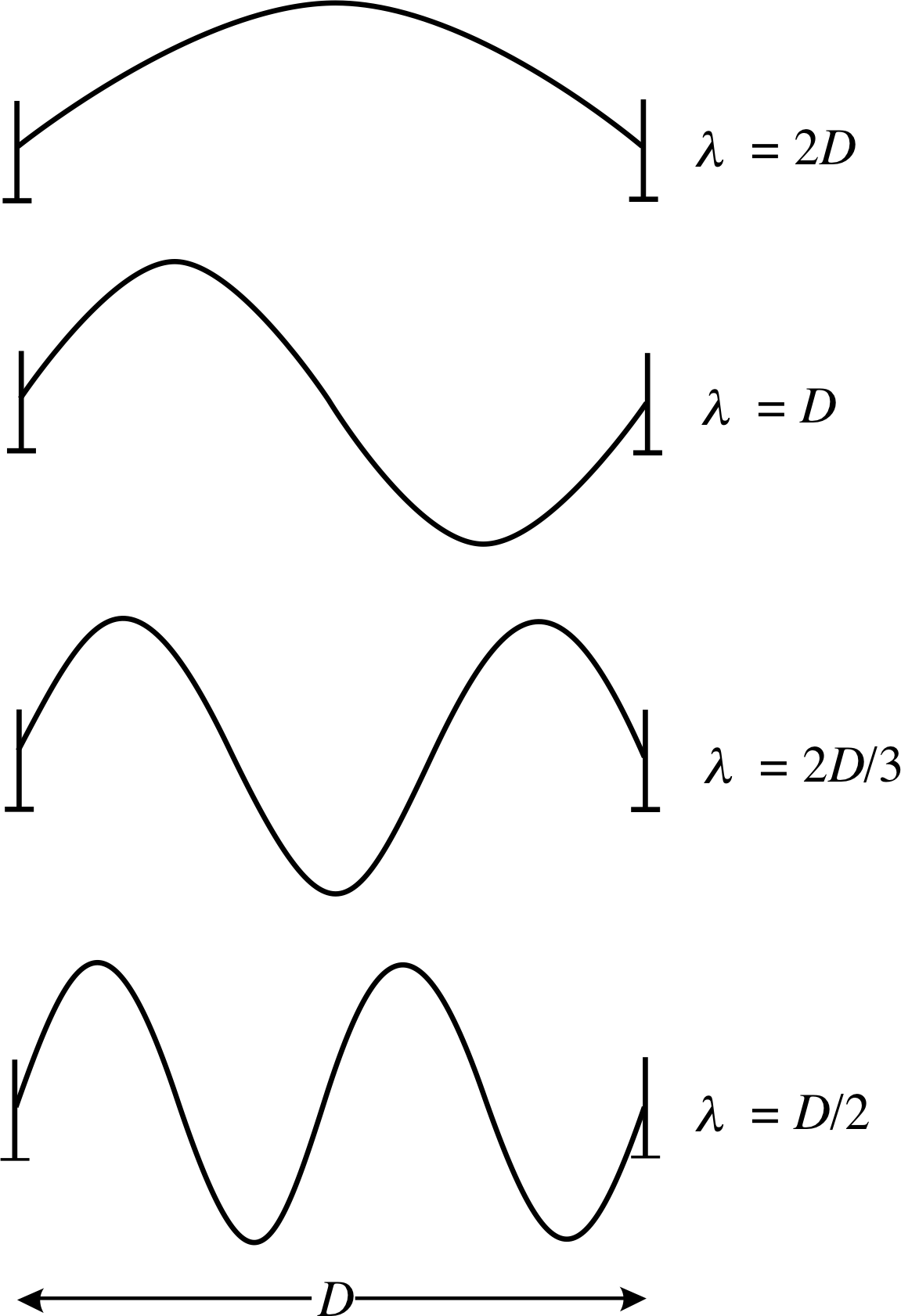
Figure 6 Four of the standing wave modes that may be set up on a taut, elastic string that is fixed at each end.
Answer F2
The wavefunction of the particle must be zero at the two end points, x = 0 and x = 5 × 10⁻¹⁴ m. Between these two points there may be any number n (a positive integer), of half wavelengths as shown in Figure 6. The expression for the spatial part of a wavefunction that satisfies these requirements is:
spatial wavefunctions: $\psi_n(x) = A_n\sin\left(\dfrac{n\pi x}{D}\right)$
where the length D is 5 ×10⁻¹⁴ m.
Question F3
What is the energy of the ground state of the particle in the previous question, if the mass of the particle is 9.1 × 10⁻³¹ kg?
Is this energy level degenerate?
Answer F3
The energy levels of a particle in this one–dimensional box are:
$E_n = \dfrac{n^2h^2}{8mD^2}$
In the ground state (n = 1) of the particle in the previous question:
$E_1 = \rm \dfrac{(6.6\times10^{-34}\,J\,s)^2}{8\times9.1\times10^{-31}\,kg\times(5.0\times10^{-14}\,m)^2} = 2.4\times10^{-11}\,J$
There is only one wavefunction (n = 1) with this energy and so the level is non-degenerate.
1.3 Ready to study?
Study comment In order to study this module you will need to be familiar with the following terms: de Broglie hypothesis, de Broglie wave, de Broglie wavelength, electron, energy, hydrogen atom (including the Bohr model), momentum, photon, Planck’s constant and quanta. You will need to be familiar with the basic characteristics of waves and wave packets, including; amplitude, frequency, wavelength, propagation speed, phase speed and group speed; and with wave phenomena such as diffraction, interference, and superposition; and to know the difference between a travelling wave and a standing wave. You also should be familiar with the differentiation and integration of simple functions of x, including exponentials and trigonometric functions. If you are uncertain about any of these terms then you can review them now by referring to the Glossary, which will also indicate where in FLAP they are developed. The following Ready to study questions will allow you to establish whether you need to review some of the topics before embarking on this module.
Question R1
A wave travelling along the x–axis consists of a moving disturbance that varies with time and position, which may be represented by a function of two variables y (x, t). The ‘shape’ of the wave at any particular time t = T is described by its wave profile at that time, y (x, T), which depends on the single variable x since T is a given constant in this case. The profile may be thought of as an instantaneous snapshot of the wave at the given time.
(a) At t = 0, the wave profile of a particular wave is given by y = A sin(kx), where k is a constant called the angular wavenumber of the wave. Write down the amplitude and wavelength of the wave.
(b) If the wave in part (a) has a frequency f, write down the general relationship between the wavelength, the frequency and the speed of the wave. If the angular frequency of the wave is ω = 2πf, write down the corresponding relationship between angular wavenumber, angular frequency and speed.
Answer R1
(a) For the wave profile y = A sin(kx), the maximum size of the displacement is referred to as the amplitude. So A is the amplitude. The wavelength is the smallest distance between points on the wave that have the same phase. The function sin θ is periodic, it repeats itself every time θ increases by 2π. Two points separated by a wavelength λ, say x and x + λ therefore must satisfy the condition k (x + λ) − kx = 2π. Therefore λ = 2π/k.
(b) The relationship between the wavelength λ, the frequency f, and the speed υ, of the wave is υ = f λ. In terms of angular wavenumber k and angular frequency ω, the speed is υ = ω/k.
Consult the Glossary for further information.
Question R2
At a particular time the transverse displacements due to two waves, acting at a common point, are y1 = 5 sin(2x) and y2 = 2 sin(2x). Use the principle of superposition to obtain the combined effect of the two waves at this time.
Answer R2
The principle of superposition states that the combined effect of the two waves acting at a point is their algebraic sum y = y2 + y2. In our case the effect is of a wave y = 7 sin(2x).
Consult principle of superposition in the Glossary for further information.
Question R3
What is the de Broglie wavelength associated with a particle with momentum magnitude 5.0 × 10⁻²¹ kg m s−1?
[Take Planck’s constant, h, to have the value 6.6 × 10⁻³⁴ J s]
Answer R3
The de Broglie hypothesis relates the momentum magnitude, p, of a particle and its de Broglie wavelength λdB, by λdB = h/p where h is Planck’s constant. In this case, therefore, the particle has a de Broglie wavelength:
$\lambda_{\rm dB} = \rm \dfrac{6.6\times10^{-34}\,J\,s}{5.0\times10^{-21}\,kg\,m\,s^{-1}} = 1.3\times10^{-13}\,m$
Consult the de Broglie hypothesis, de Broglie wavelength, and Planck’s constant in the Glossary for further information.
Question R4
Write down and evaluate the definite integral of the function f (x) = x3 between the limits x = 3 and x = 4.
Answer R4
The definite integral of the function f (x) between x = 3 and x = 4 is written $\displaystyle \int_3^4 f(x)\,dx$.
The value for our simple function is
$\displaystyle \int_3^4x^3\,dx = \left[\dfrac{x^4}{4}\right]_3^4 = \dfrac14(4^4-3^4) = 43.75$
Consult integration in the Glossary for further information.
Question R5
Give an expression for the indefinite integral $\int\sin(2x)\,dx$.
Answer R5
$ \int\sin(2x)\,dx = -\frac12\cos(2x) + \text{constant of integration}$
2 A review of basic quantum physics
2.1 Particle–like behaviour of electromagnetic radiation
Max Planck’s i interpretation (1900–) of the distribution of light emitted by an idealized hot body, the so–called black–body spectrum, provided the first evidence that the interactions of radiation with matter were quantized.
If a body is heated to a high temperature it emits light over a wide continuous range of wavelengths. When the spectrum of this radiation is examined and the relative brightness of the emission from unit area of the surface is plotted as a function of wavelength, it is found that the wavelength for peak emission and the total radiated power are determined mainly by the temperature of the body, not by its material. In the case of an ideal emitter, a so–called black body, the spectrum would be entirely determined by the temperature. An explanation for the detailed shape of the black–body spectrum proved impossible using classical physics, which predicted that the brightness should increase without limit at high frequencies. Planck was able to resolve this by assuming a quantum model for the interaction of matter and radiation. In particular he assumed that the interaction involved the emission and absorption of quanta, (which later become known as photons) with energy hf, where f is the frequency of the radiation and h is Planck’s constant. The spectrum predicted on the basis of this assumption was in excellent agreement with the observed spectrum of black–body radiation. i
More direct evidence for photons was provided later through the photoelectric effect and the Compton effect. In the photoelectric effect, electrons are produced by shining ultraviolet radiation on to a metal surface. It is found that the maximum kinetic energy of the photoelectrons emitted from any particular surface depends only on the frequency of the incident radiation and not on the intensity of the radiation. In addition, there is a threshold frequency for a particular material and no photoelectrons are produced below this frequency, however intense the radiation. Classical wave models of electromagnetic radiation could not explain this and it was left to Einstein to interpret the observed behaviour in terms of a particle–like interaction between the radiation and the electrons in the material. In this interaction energy is absorbed from individual photons of discrete energy E given by:
photon energy E = hf(1)
This result became known as the Planck–Einstein formula.
Some 20 years later, a crucial series of experiments, involving the scattering of X–rays by different targets showed that the scattered X–rays had a slightly longer wavelength (or a lower frequency) than the incident radiation and also that the shift in wavelength depended on the scattering angle. These observations were inexplicable using classical wave ideas. However, Arthur H. Compton (1892–1962) gave a quantum interpretation of these results, which involved the photon having a momentum as well as the energy given by Equation 1. (The collision between the X–ray photon and an essentially free electron in the material could then be treated as a particle–particle collision, conserving energy and momentum in the usual way.) The required expression for the photon momentum magnitude was:
photon momentum p = E/c = h/λ(2)
This scattering phenomenon later became known as the Compton effect.
2.2 Wave–like behaviour of matter
The next stage in the evolution of quantum physics came when Louis de Broglie (1892–1987) suggested that since the particles (i.e. photons) which make up electromagnetic radiation can exhibit wave–like behaviour, perhaps the same is true of every other particle. This suggestion became known as the de Broglie hypothesis, and the wave associated with a particle, the de Broglie wave, was expected to have its de Broglie wavelength set by the magnitude of the momentum p of the particle, according to the expression:
de Broglie wavelength λdB = h/p(3)
The suggestion that particles of matter might exhibit wave–like behaviour implies that such particles might exhibit diffraction and interference. If so, the closely spaced planes of atoms in a crystalline solid might be used to diffract the de Broglie waves associated with an electron beam with particle energies of a few tens of electron volts. Such an experiment was carried out in 1927 by C. H. Davisson and L. H. Germer and they obtained a diffraction pattern in good agreement with de Broglie’s predicted wavelength. Subsequently, many other experiments have demonstrated that all particles, irrespective of charge, mass, shape or composition, produce a diffraction pattern which is consistent with the de Broglie hypothesis.
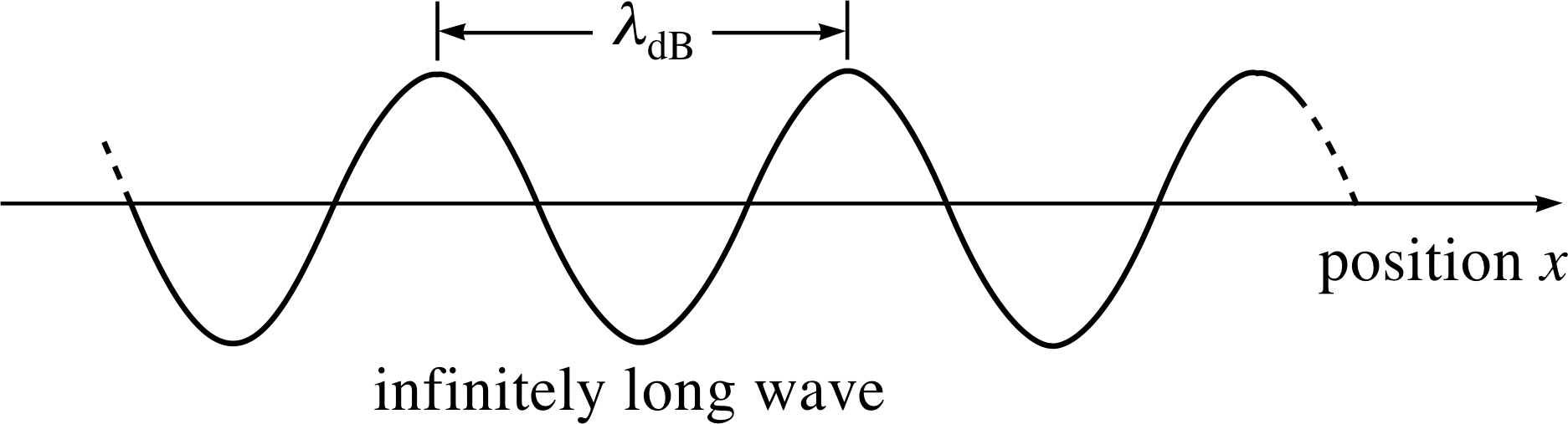
Figure 1 The profile of a de Broglie wave of fixed amplitude and wavelength λdB, corresponding to a particle moving in the positive x–direction with momentum px. Note that the figure shows a snapshot of the wave, which is actually travelling in the positive x–direction.
Figure 1 shows an instantaneous snapshot of the de Broglie wave for a particle with definite momentum px travelling along the x–direction.
The precise nature of de Broglie waves and the exact sense in which such waves are to be associated with particles was left unclear by de Broglie. However, subsequent work by others, notably Erwin Schrödinger (1887–1961), Werner Heisenberg (1901–1976) and Max Born (1882–1970), put de Broglie’s ideas onto a firmer mathematical footing and eventually brought about a complete revolution in physical thinking. Part of that revolution forms the main theme of this module, and we will come to it later. i
In the meantime, we will continue to use the term ‘de Broglie wave’ to describe the wave aspect of a particle, and we will summarize later work by saying that the de Broglie wave of a particle determines the relative likelihood of detecting the particle in any given region of space. In particular, continuing to use this somewhat over–simplified language, we can say that the probability of finding a particle in any small region of space is proportional to the square of the amplitude of the de Broglie wave in that region. In this sense the disturbance that constitutes a de Broglie wave may be thought of as a disturbance in the probability of finding the associated particle.
A simple one–dimensional de Broglie wave of fixed amplitude and wavelength, extending to infinity along the x–direction, corresponds to a particle whose momentum magnitude is perfectly known. Unfortunately, such a wave is not localized in space; its amplitude is the same everywhere, and so it conveys no information at all about the position of the particle. If we wish to produce a wave of finite extent, with some implied localization of the particle, then we must construct a wave packet by superposing (adding) waves, and arrange for this superposition to diminish sharply outside the expected range of particle positions ∆x. In discussing this process it is convenient to use as the variable the angular wavenumber k rather than the wavelength λ – the two are related by
angular wavenumber k = 2π/λ(4)
Question T1
At time t = 0, the instantaneous profiles of two de Broglie waves are ψ1(x) = A1 cos(k1x) and ψ2(x) = A2 cos(k2x). i These expressions show that the two are in phase at x = 0.
(a) Write down an expression for the profile of their superposition at t = 0 and give its value at x = 0.
(b) What are the values of x closest to zero for which ψ1(x) and ψ2(x) are exactly out of phase (in anti-phase) at t = 0? Express this value of x in terms of the difference in momentum of the corresponding particles.
Answer T1
(a) The superposed wave profile is:
ψ (x) = [ψ1(x) + ψ2(x)] = A1 cos(k1x) + A2 cos(k2x)
At x = 0 we have ψ (0) = [ψ1(0) + ψ2(0)] = A1 + A2.
(b) The waves are in anti–phase when the arguments of the two cosine functions differ by any odd multiple of π. The smallest values of x for which this occurs are when the arguments differ by π so that k1x = k2x ± π, thus, using p = hk/2π:
x = ±π/(k1 − k2) = ± h/[2(p1 − p2)]
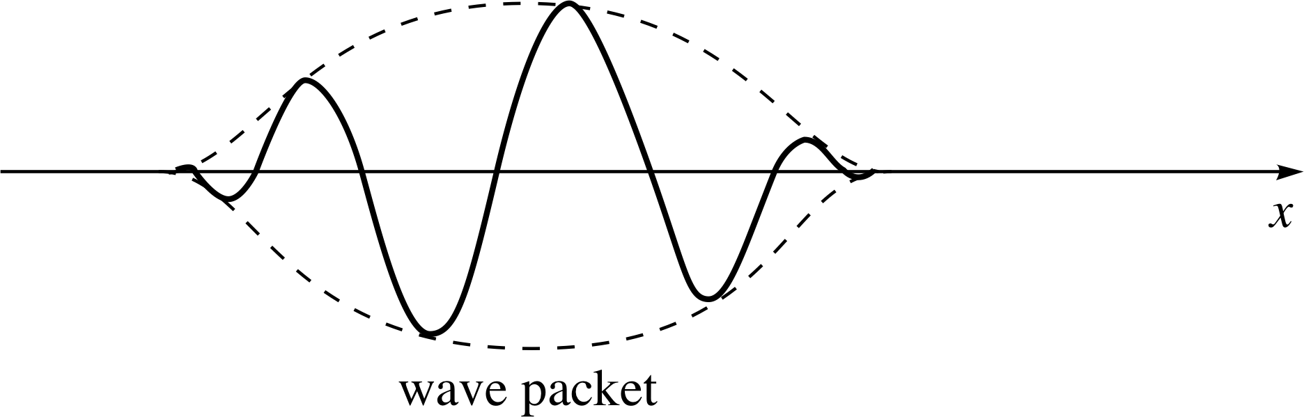
Figure 2 A wave packet constructed from a superposition of de Broglie waves of different wavelength. Again, note that the figure shows a snapshot of the wave, which is actually travelling since it describes the motion of particles. Note that although the figure shows an isolated wave packet the pattern is actually repeated all along the x–axis.
The answer to Question T1 illustrates the principle that a more localized profile can be produced by superposing two other profiles, corresponding to two different angular wavenumbers, i.e. two different momenta, by using ψ (x) = [ψ1(x) + ψ2(x)] as a new wave profile.
Such a case is illustrated in Figure 2. The answer also shows that a position of constructive interference is separated from a position of destructive interference by a distance ∆x which is determined by the angular wavenumber difference ∆k. The two quantities ∆x and ∆k being inversely related: ∆k ≈ ±π/∆x.
We can go further than this, and use more than two waves in the superposition, as shown in Figure 3. This figure shows an example of the construction of a finite wave packet by the superposition of (in this case eight) waves of suitably chosen amplitudes and wavelengths. Although each contributing wave has a well defined wavelength and associated momentum, the resultant superposition does not.
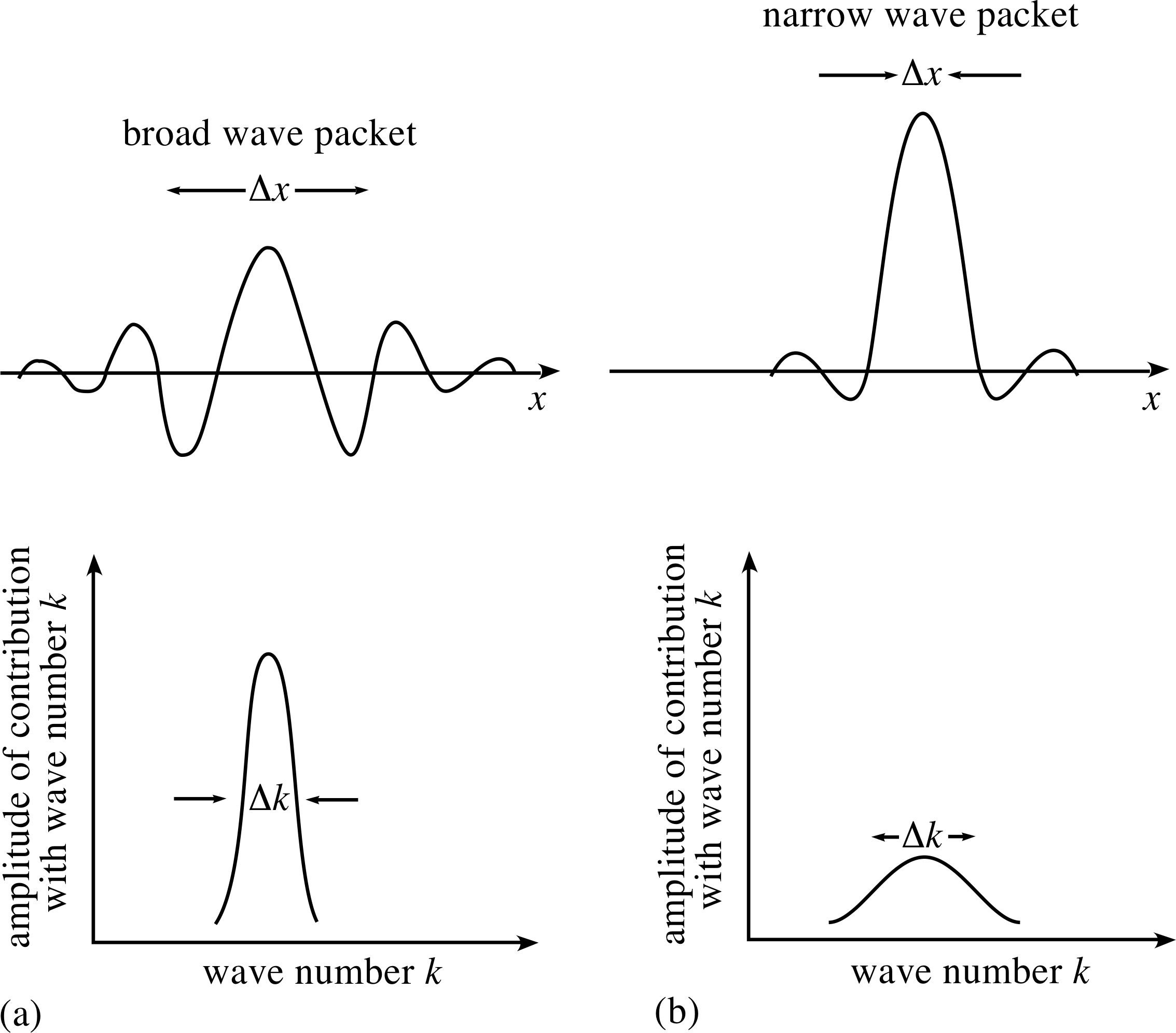
Figure 4 A broad wave packet can be constructed from the superposition of waves with a narrow range of angular wavenumbers. Conversely a narrow wave packet requires a broad range of angular wavenumbers for its construction.
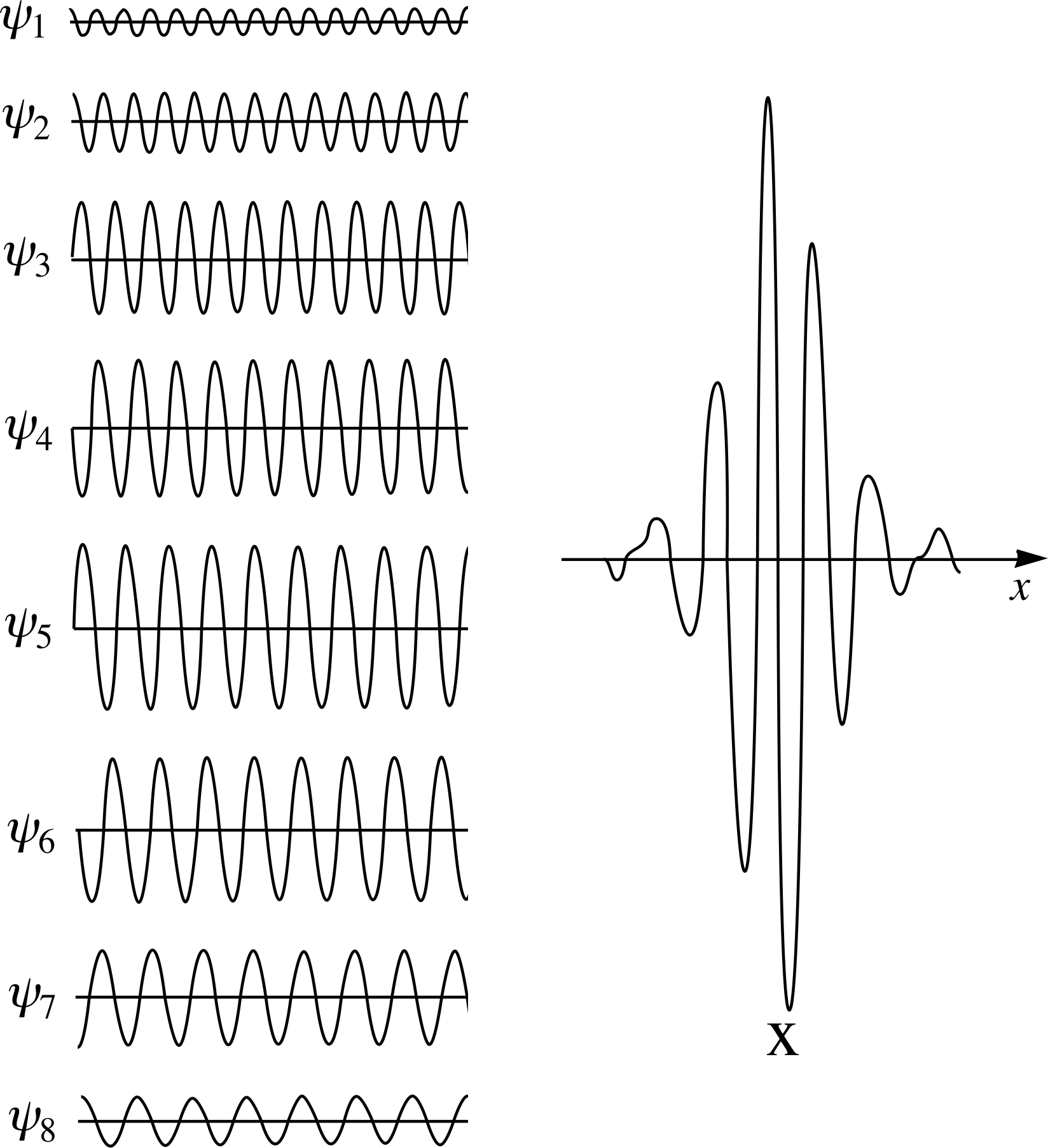
Figure 3 The localization of the wavefunction produced when eight waves with different amplitudes and wavelengths are added together using the principle of superposition.
The basic features arising from the mathematics are illustrated in Figure 4. It should be noted, in particular, that in order to localize the wave packet within a smaller and smaller region of space, there must be included in the superposition a wider and wider range of values of angular wavenumber for the contributing waves.
The greater the spread of angular wavenumbers ∆k, the narrower the width ∆x, of the corresponding wave packet.
Fourier analysis i quantifies this relationship in the simple expression:
∆x ∆k ≈ 1(5)
Notice that Equation 5 is not given as an equality since, as you will see by looking at Figure 4, ∆x and ∆k are only approximate measures of spread and have not been defined precisely. This relationship is very important however, as it shows a trend which is always satisfied, irrespective of the shape of the wave packet.
In the context of a de Broglie wave packet, each of the superposed waves will have a different de Broglie wavelength,
de Broglie wavelength λdB = h/p(Eqn 3)
and hence a different associated particle momentum. A spread in angular wavenumber will therefore correspond to a spread in particle momentum. This implies that the wave packet corresponding to a particle whose position is known to within ∆x must be composed of de Broglie waves associated with particle momenta in the range
$\Delta p = \dfrac{h}{2\pi}\Delta k \approx \dfrac{h}{2\pi}\dfrac{1}{\Delta x}$
This leads to the Heisenberg uncertainty principle:
Heisenberg uncertainty principle $\Delta x\,\Delta p_x \gtrsim \dfrac{h}{2\pi}$(6) i
where ∆px represents the irreducible uncertainty in the x–component of the momentum of a particle that is known to be localized within ∆x.
Notice that we have replaced the approximation sign in Equation 5 by a ‘greater than or approximately equal to’ sign in Equation 6 to signify that in any experiment we can never obtain simultaneous information on position and momentum in a given direction to a precision which is better than the fundamental limit set by the wave nature of matter.
Question T2
In each of the two cases below, measurements are made simultaneously of position x, and x–component of momentum px. In each case the uncertainty ∆x, is given. Estimate the percentage uncertainty in the momentum due to the Heisenberg uncertainty principle. Take Planck’s constant h, as 6.6 × 10⁻³⁴ J s.
(a) A bullet of mass 0.10 kg is travelling with a speed of 1.5 km s−1 and ∆x is 0.10 mm.
(b) A proton of mass 1.7 × 10⁻²⁷ kg is travelling with a speed of 1.0 km s−1 for which ∆x is 1.0 × 10⁻¹⁰ m.
Answer T2
(a) For the bullet, the momentum is:
px = mυx = 0.10 kg × 1.5 × 103 m s−1 = 1.5 × 10² kg m s−1
The uncertainty in position is ∆x = 1.0 × 10⁻⁴ m. The Heisenberg uncertainty principle,
Heisenberg uncertainty principle $\Delta x\,\Delta p_x \gtrsim \dfrac{h}{2\pi}$(Eqn 6)
will give an estimate of ∆px as:
$\Delta p_x \gtrsim \dfrac{h}{2\pi\Delta x} = \rm \dfrac{6.6\times1^{-34}\,J\,s}{2\pi\times1.0\times10^{-4}\,m} = 1.1\times10^{-30}\,kg\,m\,s^{-1}$
The percentage uncertainty is:
$\dfrac{100\Delta p_x}{p_x}\% = \dfrac{100\times1.1\times10^{-30}}{1.5\times10^2}\% = 7.3\times10^{-31}\%$
(b) For the proton the momentum is:
px = mpυx = 1.7 × 10−27 kg × 1.0 × 103 m s−1 = 1.7 × 10⁻²⁴ kg m s−1
For ∆x = 1.0 × 10⁻¹⁰ m:
$\Delta p_x \gtrsim \dfrac{h}{2\pi\Delta x} = \rm \dfrac{6.6\times10^{-34}\,J\,s}{2\pi\times1.0\times10^{-10}\,m} = 1.1\times10^{-24}\,kg\,m\,s^{-1}$
The percentage uncertainty is:
$\dfrac{100\Delta p_x}{p_x}\% = \dfrac{100\times1.1\times10^{-24}}{1.7\times10^{-24}}\% = 65\%$
We are now in a position to introduce the concept of a wavefunction and to begin the journey from the old de Broglie world to the new world of quantum mechanics. Our first task is to organize our vocabulary. So far, we have sometimes referred to electrons, protons, neutrons and other such entities rather loosely as ‘particles’. On other occasions we have had to accept that they exhibit wave–like behaviour. Neither the word ‘particle’ nor ‘wave’ conveys the full picture of their behaviour, so we will describe each of them simply as a quantum, indicating that they are neither waves nor particles but may exhibit features of either. i This is a new technical definition of the term. It is natural then to describe the study of the motion and the interaction of these quanta as quantum mechanics. This new world of quantum mechanics is a good deal more mathematical than the old world of de Broglie waves, but we will try to maintain the contact with de Broglie waves as long as we can.
3 The wavefunction for a free particle
The principles of quantum mechanics were introduced in a series of papers by Heisenberg, Schrödinger, Born and Pascual Jordan (1902–1980) in the years 1925–1926. Initially there were two quite distinct formulations of quantum mechanics, but they were soon shown to be mathematically equivalent and Schrödinger’s version (now known as wave mechanics) now provides the usual route of entry to the subject.
Central to Schrödinger’s approach is a mathematical quantity called the wavefunction. This quantity varies with time and position, just like a wave, and replaces the more primitive (and ill-defined) concept of a de Broglie wave. It is conventional to use the upper–case Greek letter Ψ (pronounced ‘psi’) to represent the wavefunction, so in a one–dimensional problem where its value depends on position x and time t, the wavefunction is usually written Ψ (x, t). The precise form of the wavefunction in any given situation is determined by solving a (complicated) equation known as the time-dependent Schrödinger equation. Learning how to formulate this equation to represent a given physical situation is an important skill, as is learning how to solve it, but we will not be concerned with either of those issues in this module. Instead, we will concentrate on the significance and physical interpretation of the wavefunctions that satisfy it.
In the conventional interpretation of quantum mechanics the wavefunction provides the most complete description of the behaviour of a system we can hope to have. This sounds rather grand, and it certainly has far reaching implications, but in practice we are often restricted to dealing with such simple systems that even their ‘complete description’ is fairly straightforward. In the case of a particle moving in one dimension, for instance, it usually boils down to knowing the energy and momentum, and something about the relative likelihood of finding the particle in various regions.
An important mathematical property of the wavefunction Ψ (x, t) that clearly distinguishes it from a de Broglie wave is that it is generally a complex quantity. That is to say, given particular values for the variables x and t, the corresponding value of the wavefunction will generally be complex number and may therefore be written in the form
Ψ (x, t) = a + ib i
where a and b are ordinary (real) numbers and i is a special algebraic quantity, usually referred to as the square root of −1, with the property
i2 = −1
Complex numbers are used in many parts of physics, but often only as a convenience. In quantum mechanics, however, they play an essential role and are unavoidable. In this particular module we will use them as little as possible, but even here we cannot avoid them completely and you will certainly need to know more about them if you intend to pursue the study of quantum mechanics.
For the moment, the one additional fact you need to know about any complex quantity is that it may always be associated with a unique real number called its modulus_of_a_complex_numbermodulus. The modulus of Ψ (x, t) = a + ib is written | Ψ (x, t) | and is defined in the following way
ifΨ (x, t) = a + ib
then | Ψ (x, t) | = (a2 + b2)1/2
In quantum mechanics the modulus of the wavefunction plays the role that we earlier (and over-simplistically) assigned to the square of the amplitude of a de Broglie wave. In other words, if the behaviour of a quantum is described by the wavefunction Ψ (x, t)
The probability of finding the particle within the small interval ∆x around the position x at time t is
∝ | Ψ (x, t) |2 ∆x(7) i
There are several points to note here:
- Since | Ψ (x, t) | is a real quantity (it doesn’t involve i), it must be the case that | Ψ (x, t) |2 is positive. It is therefore at least possible that | Ψ (x, t) |2 might represent a probability, since probabilities are represented by real numbers in the range 0 to 1 with 0 for no possibility and 1 for certainty.
- Since ∆x is taken to be very small, | Ψ (x, t) |2 can be thought of as the probability per unit length, or probability density around position x. i
- | Ψ (x, t) |2 ∆x is a statistical indicator of behaviour. Given a large number of experiments to measure the position of a particle, set up under identical conditions, it represents the fraction of those experiments that will indicate a particle in the range ∆x at a time t. The set up for the experiment is fixed but the results of individual experiments are not always the same.
- We may write an equality sign in place of the proportionality sign in Equation 6, provided we choose an appropriate scale of probability. For the moment, we do not need to be concerned with this refinement, but we will return to it in Subsection 4.2 when we discuss normalization.
Our task now is to introduce the appropriate wavefunctions for some simple situations and to determine how these wavefunctions may be used to obtain the characteristic properties of the associated particle – such as its position, momentum and kinetic energy. We begin with the case of a free particle.
3.1 A complex travelling wave to represent a free particle
If we are to represent a moving particle by a wave then it is reasonable to use a travelling wave and so we begin by reviewing how we represent a classical travelling wave, such as a transverse wave on a string. i
A classical travelling wave on a string
A wave travelling along a string is characterized by having an amplitude A, frequency f, angular frequency ω = 2πf, wavelength λ and angular wavenumber k = 2π/λ. i When such a wave propagates in the positive x–direction, the wave displacement y (x, t) can be represented by:
travelling wave y (x, t) = A cos(kx − ωt)(8) i
The wave represented by Equation 8 can be shown to be travelling in the positive x–direction, using the following argument. Consider the position of the wave at two times t = 0 and t = ∆t, where ∆t is very short compared to the period of the wave.
At t = 0: y (x, 0) = A cos(kx) and the wave has a maximum at x = 0. At t = ∆t: y (x, ∆t) = A cos(kx − ω ∆t) and the wave has a maximum when (kx − ω ∆t) = 0. This maximum occurs at x = ω ∆t/k.
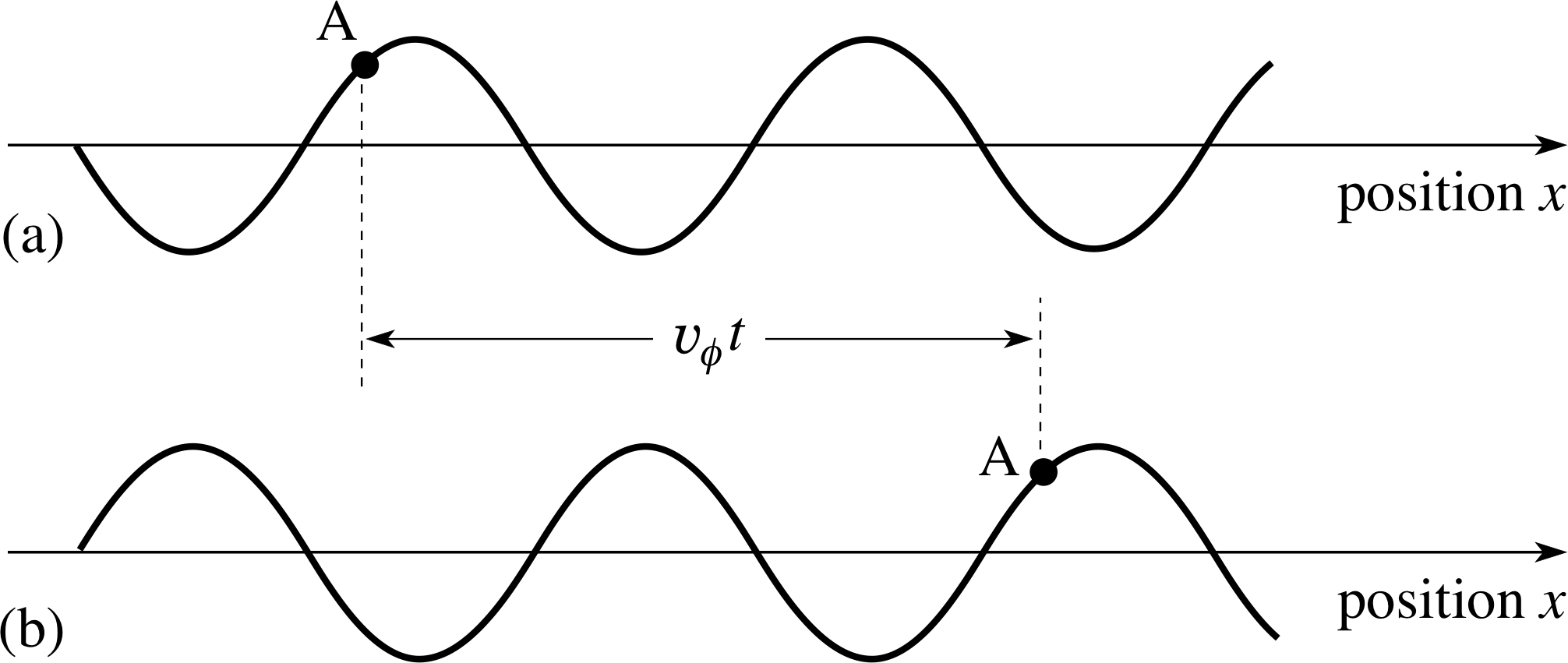
Figure 5 (a) An infinitely long wave at time t = 0. (b) The same wave at a later time t; the speed of the wave is υϕ from left to right so the wave has moved a distance υϕt to the right, but its shape is unchanged.
We deduce that the maximum of the wave has moved a distance ∆x = ω ∆t/k in the time ∆t. It is apparent that the wave is travelling along the positive x–direction and that a point of fixed phase (e.g. a point of maximum displacement where kx − ω∆t = 0) advances with a phase speed υϕ given by:
wave phase speed: υϕ = ∆x/∆t = ω/k(9)
We could rewrite Equation 8 in terms of the wave phase speed as:
travelling wave y (x, t) = A cos[k (x − υϕt)](10)
This expression for the travelling wave makes the role of the phase speed clear.
The travelling wave is shown in Figure 5.
Question T3
Obtain an expression similar to Equation 8,
travelling wave y (x, t) = A cos(kx − ωt)(Eqn 8)
but representing a wave travelling in the negative x–direction.
Answer T3
An expression for the wave travelling in the negative x–direction can be found by noting that at time ∆t the maximum displacement must be positioned at x = −ω ∆t/k.
We can achieve this simply by replacing the negative sign in the argument of Equation 8,
travelling wave: y (x, t) = A cos(kx − ωt)(Eqn 8)
by a positive sign to obtain:
y (x, t) = A cos(kx + ωt)
A quantum travelling wave in one dimension
We can now write down the wavefunction of a freely moving quantum travelling in the +x–direction. (Remember, this is found by solving the time dependent Schrödinger equation, though we will not go into that in this module.)
free particle wavefunction Ψ (x, t) = A cos(kx − ωt) + iA sin(kx − ωt)(11) i
As you can see, it owes a great deal to the expression for a one–dimensional travelling wave (Equation 8),
travelling wave y (x, t) = A cos(kx − ωt)(Eqn 8)
but there is also a striking difference. This wavefunction involves i, the square root of −1, and is therefore intrinsically complex. We will examine the significance of this in a moment, but for the present let us exploit the similarities with a travelling wave.
As you might expect the total energy, the momentum and the kinetic energy of the quantum can all be expressed in terms of the parameters ω and k of the wavefunction, through Equations 1 and 3, as:
total energy:$E = hf = \dfrac{h\omega}{2\pi} = \hbar\omega$(12) i
momentum:$p_x = \dfrac{h}{\lambda_{\rm dB}} = \dfrac{hk}{2\pi} = \hbar k$(13)
kinetic energy:$E_{\rm kin} = \dfrac{m\upsilon_x^2}{2} = \dfrac{(m\upsilon_x)^2}{2m} = \dfrac{p_x^2}{2m} = \dfrac{\hbar^2k^2}{2m}$(14)
Where we have introduced the shorthand $\hbar$ for the commonly met quantity h/2π. Notice an important feature of quantum mechanics shown here – the properties of the quantum are derivable from the mathematical form of its wavefunction, in this case simply by inspection of the coefficients of x and t.
Now, let us see what information about the position of the quantum, can be derived from the wavefunction of Equation 11.
Using the general expression for the modulus of a complex quantity we see that in this case
| Ψ (x, t) | = [A2 cos2(kx − ωt) + A2 sin2(kx − ωt)]1/2
But sin2θ + cos2 θ = 1 for all values of θ
So| Ψ (x, t) | = A
and| Ψ (x, t) |2 = A2(15)
Thus, the probability density is independent of x, and the likelihood of finding the quantum in a small region of fixed length ∆x is the same everywhere. You shouldn’t be surprised by this result: in the first place there is no reason why a freely moving quantum should be more likely to be found in one place than another; secondly this quantum has a well defined momentum magnitude so ∆p = 0 and it follows from the uncertainty principle that $\Delta x (=\hbar/\Delta p)$ will be undefined.
We might now be tempted to calculate the phase velocity from the wavefunction in Equation 11,
free particle wavefunction Ψ (x, t) = A cos(kx − ωt) + iA sin(kx − ωt)(Eqn 11)
When we do so we are in for a shock! By analogy with the wave on a string we find the phase speed of this wavefunction is:
phase speed: $\upsilon_\phi = \dfrac{\omega}{k} = \dfrac Ep = \dfrac{\frac12m\upsilon^2}{m\upsilon} = \dfrac{\upsilon}{2}$(16)
In Equation 16 we have used the usual expressions for the kinetic energy and momentum magnitude of a particle travelling with speed υ. We have arrived at the disturbing conclusion that the phase speed of the wavefunction is not the same as the velocity of the associated particle, but half this value! We will resolve this apparent paradox in the next subsection.
3.2 A travelling wave packet to represent a free particle
Just as we were able to construct a wave packet from de Broglie waves to represent a localized particle, so too we can produce a localized wavefunction by superposing free particle wavefunctions like that of Equation 11,
free particle wavefunction Ψ (x, t) = A cos(kx − ωt) + iA sin(kx − ωt)(Eqn 11)
If this quantum wave packet moves through space, its motion can represent the motion of the associated free particle. Of course, since the wave packet will involve a range of angular wavenumbers it will not describe a particle with precisely determined momentum but that, according to the uncertainty principle, is the price we must pay for having some idea where the particle is located.
When the phase speed of a wave depends on its wavelength or angular wavenumber, individual waves of a given k will move with different phase speeds whilst the wave packet itself will travel at the group speed. According to classical wave theory the group speed is the speed with which the energy is propagated and is given by the expression:
group speed: υg = dω/dk(17) i
We will soon use Equation 17 to investigate the group speed of our quantum wave packet. However, before we do that let us clarify the meaning of the equation by using it to investigate a packet of (hopefully familiar) electromagnetic waves.
Group speed of an electromagnetic wave packet in a vacuum
For an electromagnetic wave of frequency f and wavelength λ travelling in a vacuum:
c = f λ(18)
so the phase speed of a single electromagnetic wave is
phase speed: $\upsilon_\phi = \dfrac{\omega}{k} = \dfrac{2\pi f}{2\pi/\lambda} = f\lambda = c$(19)
The phase speed is constant, it is independent of k, and ω = kc. In a vacuum, an electromagnetic wave packet composed of many such waves with different values of k moves with an overall speed known as its group speed, given by
group speed: $\upsilon_{\rm g} = \dfrac{d\omega}{dk} = \dfrac{d}{dk}(ck) = c$(20)
Since the group speed is also c, the wave packet travels at the same speed as each of the constituent waves within it. The wave packet thus travels through a vacuum without change of shape.
In a medium the situation is rather different. If an electromagnetic wave packet travels through any material, other than vacuum, the phase speed of each constituent wave is reduced by the refractive index, which usually depends on k. In this case, the group speed and the various phase speeds differ and the wave packet changes its shape and spreads out as it propagates. This process is called dispersion. and the relation between ω and k is called the dispersion relation of the material.
Group speed of a quantum wave packet
To determine the group speed of the quantum wave packet representing a free particle we first need to determine its dispersion relation (i.e. the relationship between ω and k). We can do this by recognizing that for a free particle the total energy and the kinetic energy must be identical since it then follows from Equations 12 and 14,
total energy:$E = hf = \dfrac{h\omega}{2\pi} = \hbar\omega$(Eqn 12)
kinetic energy:$E_{\rm kin} = \dfrac{m\upsilon_x^2}{2} = \dfrac{(m\upsilon_x)^2}{2m} = \dfrac{p_x^2}{2m} = \dfrac{\hbar^2k^2}{2m}$(Eqn 14)
that:
quantum dispersion relation: $\omega = \dfrac{\hbar k^2}{2m}$(21)
so:
quantum group speed: $\upsilon_{\rm g} = \dfrac{d\omega}{dk} = \dfrac{d}{dk}\left(\dfrac{\hbar k^2}{2m}\right) = \dfrac{\hbar k}{m} = \dfrac{p_x}{m} = \upsilon_x$(22)
We thus find that for a quantum wave packet, the group speed with which the packet moves (i.e. speed with which the energy is transmitted) is equal to the speed of the associated particle. This resolves the problem we had at the end of Subsection 3.1, where we wrongly associated particle speed with phase speed rather than group speed.
Question T4
An electromagnetic wave packet moves through a material in which the dispersion relation is:
k = bω (1 + aω)
where a and b are positive constants. Obtain expressions for: (a) the phase speed and (b) the group speed of the wave packet.
Which of these two speeds is the greater?
Answer T4
(a) The phase speed is given by Equation 19,
phase speed: $\upsilon_\phi = \dfrac{\omega}{k} = \dfrac{2\pi f}{2\pi/\lambda} = f\lambda = c$(Eqn 19)
$\upsilon_\phi = \dfrac{\omega}{k} = \dfrac{\omega}{b\omega(1+a\omega)} = \dfrac{1}{b(1+a\omega)}$
(b) The group speed is given by Equation 17,
group speed: υg = dω/dk(Eqn 17)
$\upsilon_{\rm g} = \dfrac{d\omega}{dk} = \left(\dfrac{dk}{d\omega}\right)^{-1} = (b+2ab\omega)^{-1} = b(1+2a\omega)^{-1} = \dfrac{1}{b(1+2a\omega)}$
If a and b are positive constants, the denominator is larger in the second expression and so the phase speed is the greater.
4 The wavefunction for a particle confined in one dimension
We now turn our attention from freely moving particles (whether localized or not) to particles that are confined to a limited region of the x–axis. As with the travelling wave examples discussed earlier, we will approach the quantum wave problem through the familiar territory of classical waves, and we start by considering standing waves.
4.1 A particle confined in a one–dimensional box
A classical standing wave on a string
The simplest classical example of a one–dimensional standing wave is that of a vibrating string with fixed ends, such as occurs on the string of a musical instrument. For simplicity, we consider an elastic string which, in its rest state, is straight and taut with length D. It is fixed at each of its ends but may be made to vibrate at right angles to its length, if disturbed – for example, by plucking. A short while after being disturbed, a standing wave becomes established on the string and this wave can be analysed in terms of a superposition of oppositely directed travelling waves with various amplitudes; i this result can again be understood mathematically in terms of a Fourier superposition.
The significant difference between the free moving wave packet, discussed in Subsection 3.2, and the standing wave here, is that the wavelengths involved in the superposition can now have only certain particular values and do not form a continuous range.
Figure 6 Four of the standing wave modes that may be set up on a taut, elastic string that is fixed at each end.
The origin of this restriction on the contributing wavelengths is easy to explain. Since the end points of the string are fixed the displacement of the string must be zero at either end. These are known as the boundary conditions on the standing wave, and all the travelling waves that contribute to the superposition must obey them. In this case, the boundary conditions of zero displacement require that the standing wave can be expressed as a sum of travelling sine waves of definite wavelengths and amplitudes.
The particular wavelengths allowed are those for which an integer number of half wavelengths fits into the distance D, between the ends of the string.
Figure 6 shows ‘freeze-frame’ snapshots of some of these simplest standing waves that can arise. These elemental oscillations are known as the standing wave modes of the string. It is possible to excite a single mode, with a particular initial condition, but in general, several modes may be operating at the same time. When a single mode is excited, each point on the string oscillates at the same mode frequency but with an amplitude which depends on position along the string. Positions with zero amplitude are called node_in_a_standing_wavenodes and positions with maximum amplitude are called antinodes; the ends of the string are nodes. The distance between a node and the adjacent antinode is one quarter of the wavelength for that mode. If the string is excited into single mode oscillation it will continue in that mode until it is disturbed in some way, although energy losses due to friction usually damp the oscillation away, eventually.
✦ How many half wavelengths are contained in the distance D for the wave form in the bottom picture of Figure 6?
✧ There are two whole wavelengths shown. Therefore, four half wavelengths are contained between the end points.
The vertical displacements in any one of the one–dimensional standing wave modes, shown in Figure 6, may be represented mathematically as follows:
Standing wave mode n: yn (x, t) = An sin(knx) cos(ωnt)(23)
The wavelength i of the mode n is determined by the condition:
$D = \dfrac{n\lambda_n}{2}$
for n = 1, 2, 3, 4, ... (i.e. n is a positive integer).
We can write the associated angular wavenumbers kn as:
$k_n = \dfrac{2\pi}{\lambda_n} = \dfrac{n\pi}{D}$(24)
so the modes become:
$y_n(x,\,t) = A_n\sin\left(\dfrac{n\pi x}{D}\right)\cos(\omega_n nt)$ for n = 1, 2, 3, ...(25)
For a given mode Equation 23 does not lead to a travelling wave. Each point at position x on the string undergoes oscillation at the same angular frequency ωn, but with an amplitude An sin(knx), which depends on position. At an antinode the amplitude is An. Since all points on the string oscillate in phase at the same frequency, the time dependence of this stationary wave is the same at each point and for many purposes is of less interest than the spatial dependence of the mode.
However, if we ask what happens when two or more different modes operate simultaneously then we find that a more interesting time–dependence emerges. In particular, interference between two standing waves of different frequencies produces beats i at the difference frequency and the shape of the string is no longer a fixed sinusoid. Visually, the string appears to contain travelling waves which move back and forth along it.
A quantum wavefunction for one–dimensional confinement

Figure 7a A particle of mass m is moving in the space between two parallel infinite planes, separated by a distance D, measured along the x–axis.
For our quantum example, we will again consider the simplest case of one–dimensional confinement subject to appropriate boundary conditions. The wavefunction can then be completely specified in terms of a single position coordinate (x) and a time coordinate (t). The particle is not allowed outside of a finite range of x–values, say between x = 0 and x = D.
A realization of this situation could be a particle held in the space between two parallel infinite planes, separated by a distance D, measured along the x–axis. For example, we might locate one plane at x = 0 and the other at x = D, as shown in Figure 7a. This is usually called a one–dimensional box – it is actually a box in three–dimensional space, but the confinement is in one dimension only. The confinement of the particle means that the wavefunction must be zero everywhere outside the box, so there is no probability of finding the particle outside the box. It follows from this that we require the wavefunction to fall to zero at the boundary – in this case, at the walls of the box.
Thus the wavefunction must satisfy the boundary conditions:
Ψ (0, t) = 0 and Ψ (D, t) = 0 for all t
Before we consider this system in detail, let us examine whether the uncertainty principle has anything to say about this situation. When we make a mental picture of the situation we must be careful not to imply more information than we can legitimately claim from the Heisenberg uncertainty principle.
Question T5
Could we say that, in the realization of a one–dimensional box described above, the particle has only x–motion, i.e. that this is a one–dimensional problem, since the particle has no y– or z–components of velocity? Present your argument carefully. i
Answer T5
This claim is a valid possibility. It requires υy = 0 and υz = 0, so py = 0 and pz = 0. To have this perfect knowledge of py and pz implies that ∆py and ∆pz are both zero. From the Heisenberg uncertainty principle this is only tenable providing both ∆y and ∆z are undefined, so we are allowed no information about where the particle is to be found along either the y– or z–axes. We have admitted this from the start by having the space between the plates infinite in both y– and z–coordinates, so the statement of the question offers information which is consistent with the Heisenberg uncertainty principle.
Question T6
In the situation described in Question T5, could we claim that the particle is moving along the x-axis? Present your argument carefully. i
Answer T6
This claim offers information which is inconsistent with the Heisenberg uncertainty principle and so is not a valid possibility. If we know that the particle is moving along the x–axis then we are claiming not only that py = 0 and pz = 0 but also that y = 0 and z = 0, which requires perfect knowledge of the y– and z–coordinates and hence that ∆py and ∆pz are each zero. This is not possible, from the Heisenberg uncertainty principle.
The simplest wavefunctions describing a quantum confined between x = 0 and x = D, in a one–dimensional box may be written in the form:
confined wavefunction: i
${\it\Psi}_n(x,\,t) = \psi_n(x)[\cos(\omega_nt) + i\sin(\omega_nt)] = A_n\sin\left(\dfrac{n\pi x}{D}\right)[\cos(\omega_nt) + i\sin(\omega_nt)]$ n = 1, 2, 3, ...(26)

Figure 7b/c (b) The three lowest energy stationary state wavefunctions that can describe the particle. (c) The values of | ψ (x) |2 for the three lowest energy stationary states shown in (b).
Note that these wavefunctions satisfy the boundary conditions, and that we can separate out the spatial and time dependencies, as we did for the classical wave. The part of the wavefunction that depends on position (x) is denoted by the lower case Greek letter ψ and is therefore written as ψn(x) in each case. This is called the spatial part of the wavefunction, or simply the spatial wavefunction. (Note the distinction between the wavefunction Ψn(x, t) and its spatial part ψn(x).) In this particular case:
spatial wavefunction:
$\psi_n(x) = A_n\sin(k_nx) = A_n\sin\left(\dfrac{n\pi x}{D}\right)$ n = 1, 2, 3, ...(27)
As for the classical case, the quantum wavefunctions consist of a set of modes for the system. The time–dependence is common to a particular mode and it is the spatial part of these wavefunctions which is of most interest. The spatial part of each of the first three wavefunctions, as given by Equation 27 is shown in Figure 7b. As in the classical case, if the system is excited into a particular single mode then it will continue with this same wavefunction indefinitely, unless it is perturbed in some way. These persisting single mode wavefunctions are called the stationary states of the system; they are the quantum equivalent of the modes of a classical system. Stationary states have the particular property that they correspond to a probability density | Ψn(x, t) |2 that is independent of time.
✦ Confirm that | Ψ (x, t) |2 is independent of time for these stationary states, and show that | Ψ (x, t) |2 = | ψ (x) |2.
✧ Applying the general expression for the modulus of a complex quantity to Equation 26,
${\it\Psi}_n(x,\,t) = \psi_n(x)[\cos(\omega_nt) + i\sin(\omega_nt)] = A_n\sin\left(\dfrac{n\pi x}{D}\right)[\cos(\omega_nt) + i\sin(\omega_nt)]$ n = 1, 2, 3, ...(Eqn 26)
$\lvert\,{\it\Psi}_n(x,\,t)\,\rvert^2 = A_n^2\sin^2\left(\dfrac{n\pi x}{D}\right)[\cos^2(\omega_nt) + i\sin^2(\omega_nt)] = A_n^2\sin^2\left(\dfrac{n\pi x}{D}\right) = \lvert\,\psi_n(x)\,\rvert^2$
The final modulus sign around ψn(x) is superfluous in this case since we have chosen An to be real, but in general An and hence ψn(x) may be complex, and the process of taking its modulus is then significant.
The time dependence of the nth wavefunction in Equation 26 is determined by the particle’s total energy, En through Equation 12:
total energy:$E = hf = \dfrac{h\omega}{2\pi} = \hbar\omega$(Eqn 12)
Equation 13 gives the momentum in the nth mode as:
momentum:$p_x = \dfrac{h}{\lambda_{\rm dB}} = \dfrac{hk}{2\pi} = \hbar k$(Eqn 13) i
Equation 14 gives the kinetic energy in nth mode as:
kinetic energy:$E_{\rm kin} = \dfrac{m\upsilon_x^2}{2} = \dfrac{(m\upsilon_x)^2}{2m} = \dfrac{p_x^2}{2m} = \dfrac{\hbar^2k^2}{2m}$(Eqn 14)
For this situation, there are no changes in potential energy in the box and so we may set the potential energy equal to zero everywhere in the box. This means that the kinetic energy is the same as the total energy En, which is:
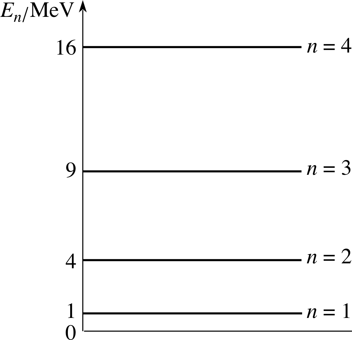
Figure 8 The first four allowed energy levels of a particle in a one–dimensional box. En = n2h2/(8mD2).
The total energy: $E_n = \dfrac{\hbar^2k_n^2}{2m} = \dfrac{\hbar^2n^2\pi^2}{2mD^2} = \dfrac{n^2h^2}{8mD^2}$(28)
where n can take on any positive integer value (n ≥ 1). These allowed values of En are known as the energy levels of the system.
Figure 8 shows the first four such energy levels. The stationary state of lowest energy is called the ground state and the associated energy level is called the ground level. States with higher energy are called excited states and their energies are excited levels. Equation 28 represents a very important and characteristic feature of quantum mechanics. It shows that, if a particle is constrained (the constraint being represented by boundary conditions on the wavefunction) then its energy may not take on any arbitrary value. Only certain discrete energies determined by the integer n in Equation 28 are permitted. The energy is said to be quantized and n is referred to as a quantum number.
4.2 Comparison between the classical and quantum cases
We have now arrived at the predictions of quantum mechanics for a particle in a one–dimensional box. These predictions are in striking conflict with classical physics so we should take time to reflect on them and draw out just how fundamental the differences are. Before we draw together the conclusions of the quantum model, let us look briefly at how classical physics would model a particle trapped between these two impenetrable walls.
Question T7
Explain how classical physics could describe a particle with fixed kinetic energy, trapped in a one–dimensional box, given that there is no motion in the y– or z–directions. Comment on the speed and direction of the motion and whether the speed or energy is restricted in any way by the box.
Answer T7
We would probably have come to the conclusion that the particle was moving parallel to the x–axis and was continually rebounding elastically at each wall successively, with the x–component of momentum being reversed at each collision.
The particle would be pictured as moving back and forwards along a single line and it could move along this line with any speed, from zero upwards, and it could have any kinetic energy (or total energy), from zero upwards.
In contrast, the summary conclusions of our quantum treatment are as follows:
- 1
-
The system has available to it certain stationary states, or discrete states, each described by the appropriate wavefunction for that state. For the nth state:
${\it\Psi}_n(x,\,t) = \psi_n(x)[\cos(\omega_nt) + i\sin(\omega_nt)] = A_n\sin\left(\dfrac{n\pi x}{D}\right)[\cos(\omega_nt) + i\sin(\omega_nt)]$
- 2
-
Each stationary state has an associated definite discrete total energy:
$E_n = \dfrac{n^2h^2}{8mD^2}$
These are known as the energy levels of the system.
- 3$\vphantom{\dfrac{h^2}{8mD^2}}$
-
The system’s lowest energy is not zero but equal to $E_1 = \dfrac{h^2}{8mD^2}$.
- 4
-
For the stationary states the wavefunctions are complex standing waves, which do not travel and so imply no particular direction of motion for the associated particle in the box.
These conclusions differ at almost every point from the classical model!
✦ The energy becomes zero if we were to set n = 0 in the expression for En. Why does this give a result which is not physically sensible?
✧ If we put n = 0 in Equation 27,
$\psi_n(x) = A_n\sin(k_nx) = A_n\sin\left(\dfrac{n\pi x}{D}\right)$ n = 1, 2, 3, ...(Eqn 27)
then we shall have ψ = 0 everywhere which implies that the probability of finding the particle is zero at every point in the box. There is no particle in the box - it has already escaped!
These claims seem outrageous (particularly points 3 and 4), but before we are tempted to abandon this quantum model as being unrealistic, we should reflect on the fact that these discrete energy levels, which are a consequence of the confinement of the particle to a given region of space, are broadly similar what is observed to happen when an electron is confined within a hydrogen atom. Indeed, it was the discrete energy levels and the fixed transitions between them which were an integral part of the Bohr model of hydrogen and which were completely inexplicable using classical physics. Clearly, our one–dimensional box doesn’t look much like a hydrogen atom, but it shows some encouraging features as an atomic model. i
Question T8
In the state n = 1, as described by Equation 28,
The total energy:$E_n = \dfrac{\hbar^2k_n^2}{2m} = \dfrac{\hbar^2n^2\pi^2}{2mD^2} = \dfrac{n^2h^2}{8mD^2}$(Eqn 28)
the kinetic energy is known exactly. Since the motion is one–dimensional this appears to imply, by Equation 14,
kinetic energy:$E_{\rm kin} = \dfrac{m\upsilon_x^2}{2} = \dfrac{(m\upsilon_x)^2}{2m} = \dfrac{p_x^2}{2m} = \dfrac{\hbar^2k^2}{2m}$(Eqn 14)
that the momentum px is known exactly. We then appear to have the particle located in x to within ∆x = D but with the momentum px known exactly (∆px = 0). Are we claiming more information than is allowed by the Heisenberg uncertainty principle? Present your argument carefully.
Answer T8
If the particle has only x–motion and we know the kinetic energy (mυx2/2 = px2/(2m)) exactly, then we know px2 exactly. However, we do not know the direction of motion of the particle and so the sign of px is not known and ∆px is not zero.
This amounts to noting that the standing wave can be considered as a superposition of two travelling waves moving in opposite directions. We could also add, as suggested in the marginal note in Subsection 4.1, that we ought really to construct a wave packet in the box and this would require a superposition of wavefunctions corresponding to different momenta. Therefore, the statement of the question is consistent with the Heisenberg uncertainty principle and so is not invalid on this basis. DTH
Location of the particle in the one–dimensional box
Now we ask where the particle is most likely to be found within the box. From the general principle given in Equation 7, the probability of finding the particle in the interval between x and x + ∆x is proportional to | Ψ (x, t) |2 ∆x. Since we are dealing with a stationary state, this is proportional to the square of the spatial part of the wavefunction, | ψ (x) |2 ∆x.
✦ At which places is the particle most likely to be detected, when in its ground state?
Figure 7b/c (c) The values of | ψ (x) |2 for the three lowest energy stationary states shown in (b).
✧ The probability of detection is proportional to | ψ1(x) |2. From Figure 7c, | ψ1(x) |2 has its maximum value at x = D/2, the mid-plane.
To find the actual numerical value of the probability near any point we must first of all normalize the wavefunction. This means that we must ensure that the total probability of finding the particle somewhere in the box is 1 (i.e. certainty). Mathematically, this implies
$\displaystyle \int_0^D \vert\,\psi_n(x)\,\rvert^2\,dx = A_n^2\int_0^D\sin^2\left(\dfrac{n\pi x}{D}\right)\,dx = 1$(29)
i.e.$\displaystyle \dfrac{A_n^2}{2}\int_0^D\left[1-\cos\left(\dfrac{2n\pi x}{D}\right)\right]\,dx = \dfrac{A_n^2}{2}\left[x - \left(\dfrac{D}{2n\pi x}\right)\sin\left(\dfrac{2n\pi x}{D}\right)\right]_0^D = A_n^2\dfrac{D}{2} = 1$
so that we must take $A_n = \sqrt{2/D\os}$ i and the normalized_wavefunctionnormalized spatial wavefunction for the state n is therefore:
normalized spatial wavefunction: $\psi_n(x) = \sqrt{\dfrac 2D}\sin\left(\dfrac{n\pi x}{D}\right)$(30) i
where n = 1, 2, 3, 4, ...
Question T9
What is the probability that a particle in the n = 5 state will be detected between x = 0 and x = +0.1D?
Answer T9
The probability, P5(0, +0.1D), that a particle in the n = 5 state will be detected between x = 0 and x = +0.1D is:
$\displaystyle P_5(0,\,+0.1D) = \int_0^{0.1D}\lvert\,\psi_5(x)\,\rvert^2\,dx$
where we must use the normalized wavefunction for state n = 5, which is:
$\psi_5(x) = \sqrt{\dfrac 2D}\sin\left(\dfrac{5\pi x}{D}\right)$
Thus the probability is:
$\displaystyle P_5(0,\,+0.1D) = \dfrac 2D \int_0^{0.1D}\lvert\,\sin^2\left(\dfrac{5\pi x}{D}\right)\,dx = \dfrac 2D\dfrac12\left[x - \dfrac{D}{10\pi}\sin\left(\dfrac{10\pi x}{D}\right)\right]_0^{0.1D}$
using the given integral.
However$\left[x - \dfrac{D}{10\pi}\sin\left(\dfrac{10\pi x}{D}\right)\right]_0^{0.1D} = \left[0.1D-\dfrac{D}{10\pi}\sin\left(\dfrac{10\pi\,0.1D}{D}\right)\right] - 0 = 0.1D$
since sin π = 0. So, finally:
$\displaystyle P_5(0,\,+0.1D) = \dfrac 2D\dfrac120.1D = 0.1$
There is thus a 10% chance of finding the particle between x = 0 and x = +0.1D.
4.3 Energy changes or transitions in the one–dimensional box i
The quantum model for a particle in a one–dimensional box shows the existence of a set of stationary states of different energy. If the particle in one of these states is unperturbed, it will remain in the state indefinitely, in just the same way that a single standing wave mode on a string will continue with fixed energy indefinitely. If either system is perturbed, for example by gaining or losing energy, then the state of oscillation will change. In the classical case, other wave modes will become excited as the energy changes; in the quantum case, the system may make a transition between stationary states as the energy changes.
In Subsection 4.2 we noted that classically, when two standing wave modes are simultaneously operating on a string, the resulting disturbance has a time dependence at the difference frequency of the two modes. Visually, the string shows the presence of a disturbance which oscillates back and forth on the string, at this difference frequency. In the quantum case, the mixing of two stationary states with different characteristic angular frequencies ωn and ωm produces a superpositionsuperposition state which is no longer a stationary state and in which the probability density consequently depends on time. If we calculate the probability of finding the particle at a given position in the box we find that the probability density oscillates at the angular_frequencyangular beat frequency | ωn − ωm |. This corresponds to a real oscillation of the particle between the walls – rather as the classical picture suggested.
Since an electron is a charged particle, any oscillation that it exhibits should, according to classical physics, be accompanied by radiation. The oscillating electron would either be radiating away its energy (emission), or gaining energy (absorption) from an incoming electromagnetic wave. It is natural, therefore, to try to associate the emission and absorption of radiation by an atom with the presence of an electron in a superposition state, mixing two stationary states of the system. At some initial time the system is in one of these two states and at some later time it will be in the other state, having made a transition between the two states; in the interim the state is a non–stationary superposition state in which the proportions of the two stationary states are changing with time. The energy change may then be associated with a photon of frequency f = | ωn − ωm |/2π, and so corresponds to energy change
∆E = hf = h| ωn − ωm |/2π = | En −Em | i
Figure 7a A particle of mass m is moving in the space between two parallel infinite planes, separated by a distance D, measured along the x–axis.
Question T10
An electron is confined in the one–dimensional box in Figure 7a.
(a) Sketch the spatial wavefunction that describes the electron when its total energy is $E = \dfrac{9h^2}{8m_{\rm e}D^2}$.
(b) Where is the electron most likely to be detected when it has this energy?
(c) If the electron makes a transition from this state to the ground state, obtain an expression for the reduction of its energy.
(d) If this energy is given out as a quantum of radiation, what will be the frequency f of its associated radiation?
Figure 7b/c (b) The three lowest energy stationary state wavefunctions that can describe the particle. (c) The values of | ψ (x) |2 for the three lowest energy stationary states shown in (b).
Answer T10
(a) The spatial wavefunction corresponding to E = 9h2/(8meD2) is given by Equation 27,
$\psi_n(x) = A_n\sin(k_nx) = A_n\sin\left(\dfrac{n\pi x}{D}\right)$ n = 1, 2, 3, ...(Eqn 27)
with n = 3 and m equal to the mass of the electron. Compare your sketch with Figure 7b (ψ3).
(b) The electron is most likely to be detected where | ψ (x) |2 is greatest. The three places can be seen in Figure 7c (ψ32).
(c) The ground state has energy E1 = h2/(8meD2). The loss of energy is therefore
$\Delta E = \dfrac{9h^2}{8m_{\rm e}D^2} - \dfrac{9h^2}{8m_{\rm e}D^2} = \dfrac{h^2}{m_{\rm e}D^2}$
(d) The radiation with frequency f has quanta with energy ∆E = hf.
Therefore$f = \dfrac{h}{m_{\rm e}D^2}$
5 A particle confined in two or three dimensions
The quantum treatment of a particle confined in one dimension has shown many encouraging features in relation to explaining the observed behaviour of an atom. The Heisenberg uncertainty principle explains why an atom is stable against collapse into the nucleus and the confined wave model predicts quantized energies of a confined electron and associates transitions between these with the emission or absorption of electromagnetic radiation. Now we need to extend the model to confinement in three dimensions.
5.1 Extension to two–dimensional confinement
We have seen from Section 4 that when a particle is confined in one dimension it may be found in certain quantum states labelled by a single quantum number, the integer n, and described by a wavefunction Ψn(x, t). Extending this idea to two dimensions means that the wavefunction must involve two spatial coordinates (e.g. x and y) as well as t. As usual, our deliberations will be guided by the classical analogue.
A classical standing wave on a square membrane
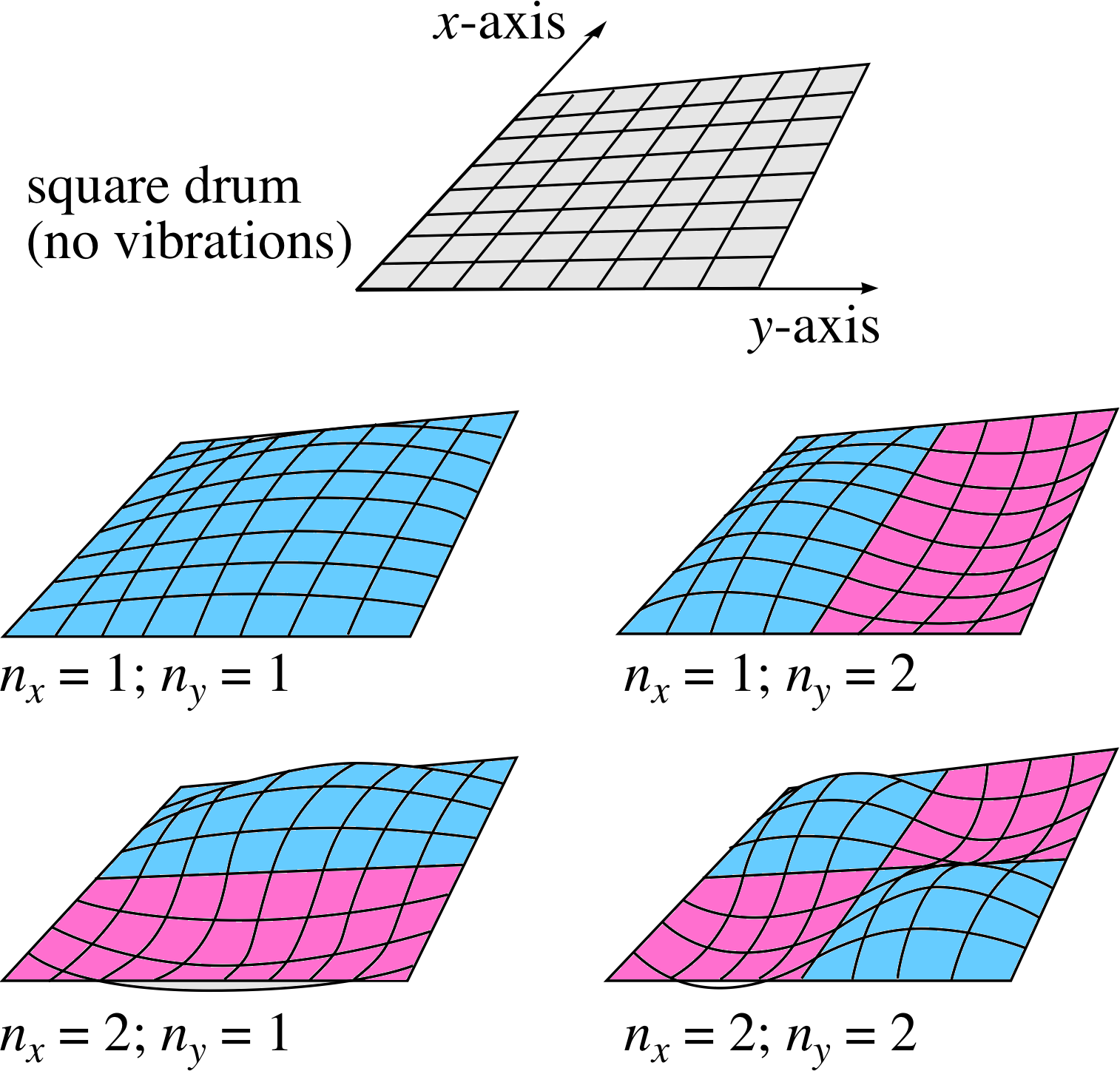
Figure 9 Four standing waves on a square, two–dimensional membrane. The integers nx and ny indicate the number of half wavelengths in the x– and y–directions, respectively.
Consider a flexible two–dimensional surface, such as a taut square drum membrane stretched over and fixed to a square framework of side D (see Figure 9). Vibrations in this surface may be set up and there will be boundary conditions in both x– and y–directions, such that there can be no vibration along the perimeter of the square.
The displacement must be zero along both the lines y = 0 (the x–axis) and y = D for any value of x between 0 and D, and along both the lines x = 0 (the y–axis) and x = D for any value of y between 0 and D. These boundary conditions are complicated to write down, but they will affect the possible vibrations of the membrane in a way that is a simple extension of the one–dimensional case.
The standing waves that can be set up will involve an integer number of half wavelengths in each of the two independent spatial dimensions. Thus there will be two integers that define a particular mode of vibration of the drum, nx for the x–direction and ny for the y–direction. This may be most clearly seen by looking at the examples shown in Figure 9.
The integers nx and ny simply designate the number of half–wavelengths of the standing wave between the two boundaries along the relevant axis. The oscillations in the two dimensions are independent in the sense that any valid value of nx can be combined with any valid value of ny to produce a valid wave mode, labelled (nx, ny) on the membrane.
A quantum wavefunction for two–dimensional confinement
We need a two–dimensional box in which to confine our particle. A realization of this might involve using two pairs of parallel infinite planes, one pair separated by a distance D along the x–axis and the other pair separated by a distance D along the y–axis. The particle is completely unrestricted in z but is confined in x and y. Because we have not constrained the particle in z (∆z is undefined) we may legitimately claim that pz = 0, or ∆pz = 0; the particle can then be said to have no motion along z, or to have only motion along x and y. These two motions will be completely independent and each will have an associated kinetic energy, with the total kinetic energy given by the sum of the two independent kinetic energies. i
Treating the two contributions to the kinetic energy as being independent will require that we use two independent quantum numbers, nx and ny, to describe each stationary state. The energy levels of those states will then be given by an extension of Equation 28:
The total energy: $E_n = \dfrac{\hbar^2k_n^2}{2m} = \dfrac{\hbar^2n^2\pi^2}{2mD^2} = \dfrac{n^2h^2}{8mD^2}$(Eqn 28)
$E_{n_x,n_y} = \dfrac{h^2}{8mD^2}(n_x^2+n_y^2)$(31)
where nx = 1, 2, 3, 4, ... and ny = 1, 2, 3, 4, ...
The corresponding spatial wavefunctions now also require two quantum numbers to label them:
$\psi_{n_x,n_y}(x,\,y) = A_n\sin\left(\dfrac{n_x\pi x}{D}\right)\sin\left(\dfrac{n_y\pi y}{D}\right)$(32)
where nx = 1, 2, 3, 4, ... and ny = 1, 2, 3, 4, ...
Compare Equations 31 and 32 with Equations 28 and 27,
$\psi_n(x) = A_n\sin(k_nx) = A_n\sin\left(\dfrac{n\pi x}{D}\right)$ n = 1, 2, 3, ...(Eqn 27)
respectively. Equation 32 obviously satisfies the boundary conditions at x = 0 and x = D and also at y = 0 and y = D.
Shared energy levels – degeneracy
Equations 31 and 32,
$E_{n_x,n_y} = \dfrac{h^2}{8mD^2}(n_x^2+n_y^2)$(Eqn 31)
$\psi_{n_x,n_y}(x,\,y) = A_n\sin\left(\dfrac{n_x\pi x}{D}\right)\sin\left(\dfrac{n_y\pi y}{D}\right)$ n = 1, 2, 3, ...(Eqn 32)
also show a feature which did not occur for the one–dimensional case. Since the energy does not depend separately on nx and ny but on the special combination (nx2 + ny2), if we exchange the values of nx and ny we leave the energy unchanged. For example, the spatial wavefunctions ψ1,2 and ψ2,1 will correspond to the same energy level even though they are different functions. When different wavefunctions share the same energy level the wavefunctions are said to be degenerate and the system is said to exhibit degeneracy. In this case we see that the degeneracy arises as a consequence of the symmetry between the x and y variables. i
| nx = 1 | nx = 2 | nx = 3 | nx = 4 | |
|---|---|---|---|---|
| ny = 1 | 2 | 5 | 10 | 17 |
| ny = 2 | 5 | 8 | 13 | 20 |
| ny = 3 | 10 | 13 | 18 | 25 |
| ny = 4 | 17 | 20 | 25 | 32 |
Table 1 shows the energies, expressed in units of h2/(8mD2), for the states ψnx,ny for a range of values of nx and ny, you should be able to see several examples of degeneracy. Degeneracies usually arise in systems with symmetries – here, it is the symmetry between the x– and y–motion. If we were to break the symmetry, for example by allowing the box to have different dimensions in x and y, we would remove the degeneracy, since the energy depends on nx2 and ny2 separately but not on (nx2 + ny2).
Symmetry and symmetry breaking are important considerations in quantum mechanics.
5.2 Extension to three–dimensional confinement
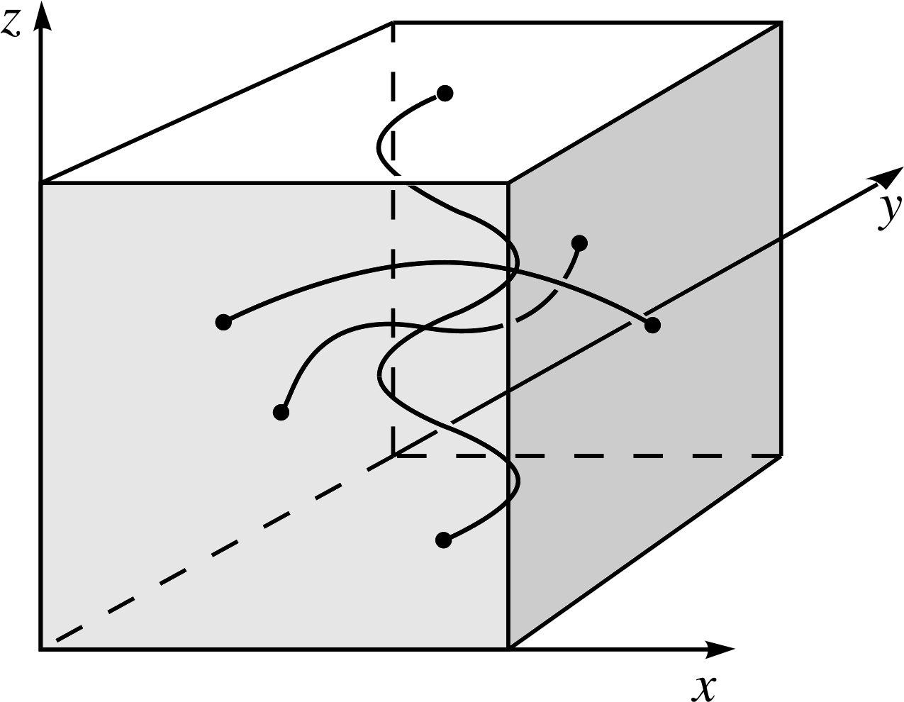
Figure 10 Standing waves confined to a cube in three dimensions. nx = 1, ny = 2 and nz = 4.
The extension to three dimensions – where the complete specification of the wavefunction of the particle requires three spatial coordinates (x, y, z) – is now straightforward. The particle is confined to a cube of side D in which standing waves may be formed, as in Figure 10. The energy levels in this case are:
$E_{n_x,n_y,n_z} = \dfrac{h^2}{8mD^2}(n_x^2+n_y^2+n_z^2)$(33)
where nx = 1, 2, 3, 4, ...; ny = 1, 2, 3, 4, ...; nz = 1, 2, 3, 4, ...
The spatial wavefunctions are:
$\psi_{n_x,n_y,n_z}(x,\,y,\,z) = A_n\sin\left(\dfrac{n_x\pi x}{D}\right)\sin\left(\dfrac{n_y\pi y}{D}\right)\sin\left(\dfrac{n_z\pi z}{D}\right)$(34)
where nx = 1, 2, 3, 4, ...; ny = 1, 2, 3, 4, ...; nz = 1, 2, 3, 4, ...
In three dimensions, a far richer range of degeneracies becomes possible. First, we have the symmetry due to the three spatial coordinates; for each set of three quantum numbers there will be six permutations of these three which give the same energy. There are also now a whole range of accidental degeneracies, based on the accidental equality of (nx2+ ny2 + nz2) for two or more sets of three quantum numbers. For example, the state nx = 8, ny = 6, nz = 5, has the same energy as the state nx = 4, ny = 3, nz = 10. There are now many cases where several independent wavefunctions share a common energy level; the number of such wavefunctions sharing a given energy level is said to be the order of degeneracy of the energy level.
Question T11
(a) Write down an expression for the energy of the ground state of a particle confined in three dimensions. Explain whether or not this state is degenerate.
(b) What is the energy of the first excited state? Is this state degenerate and, if so, what is its order of degeneracy?
Answer T11
In the general case, the energy is given by:
$E_{n_x,n_y,n_z} = \dfrac{h^2}{8mD^2}(n_x^2+n_y^2+n_z^2)$
where nx, ny, nz are positive integers.
The corresponding spatial wavefunction is given by:
$\psi_{n_x,n_y,n_z}(x,\,y,\,z) = A\sin\left(\dfrac{n_x\pi x}{D}\right)\sin\left(\dfrac{n_y\pi y}{D}\right)\sin\left(\dfrac{n_z\pi z}{D}\right)$
(a) The ground (lowest energy) state is the one for which nx = ny = nz = 1. The energy is E1,1,1 = 3h2/(8mD2). There is only one state corresponding to this energy and so the state is not degenerate. Its spatial wavefunction is given by:
$\psi_{1,1,1}(x,\,y,\,z) = A\sin\left(\dfrac{\pi x}{D}\right)\sin\left(\dfrac{\pi y}{D}\right)\sin\left(\dfrac{\pi z}{D}\right)$
(b) The second lowest energy value may be obtained in three ways. The quantum numbers are:
(1) nx = 1, ny = 1, nz = 2;
or(2) nx = 1, ny = 2, nz = 1;
or(3) nx = 2, ny = 1, nz = 1.
Each gives rise to the energy 3h2/4mD2. There are three different spatial wavefunctions:
(1) $\psi_{1,1,2}(x,\,y,\,z) = A\sin\left(\dfrac{\pi x}{D}\right)\sin\left(\dfrac{\pi y}{D}\right)\sin\left(\dfrac{2\pi z}{D}\right)$ ;
(2) $\psi_{1,2,1}(x,\,y,\,z) = A\sin\left(\dfrac{\pi x}{D}\right)\sin\left(\dfrac{2\pi y}{D}\right)\sin\left(\dfrac{\pi z}{D}\right)$ ;
(3) $\psi_{2,1,1}(x,\,y,\,z) = A\sin\left(\dfrac{2\pi x}{D}\right)\sin\left(\dfrac{\pi y}{D}\right)\sin\left(\dfrac{\pi z}{D}\right)$ ;
This energy level has an order of degeneracy of 3.
6 Closing items
6.1 Module summary
- 1
-
Indications of the particle–like behaviour of electromagnetic radiation, include evidence for the photon as a particle with energy E = hf and momentum p = E/c = h/λ.
- 2
-
Indications of the wave–like behaviour of matter, as predicted by the de Broglie hypothesis (λdB = h/p), include a variety of particle diffraction experiments. The Heisenberg uncertainty principle states that the simultaneous uncertainties in the position and momentum of a particle obey the restriction
$\Delta x\,\Delta p_x \gtrsim \dfrac{h}{2\pi}$(Eqn 6)
- 3
-
The quantum mechanical wavefunction Ψ (x, t), of a particle moving in one dimension is a complex numbercomplex quantity found by solving the time–dependent Schrödinger equation. The probability of finding the particle within the small interval ∆x around the position x at time t being ∝ | Ψ (x, t) |2 ∆x, where | Ψ (x, t) |2 is the probability density at position x.
- 4
-
An unlocalized free particle may be represented by a wavefunction of the form
ψn(x, t) = A cos(kx−ωt) + i A sin(kx−ωt)
this describes a particle for which the total energy $E = \hbar\omega$, the momemtum $p_x = \hbar k$ and the kinetic energy $E_{\rm kin}= \hbar^2k^2/2m$.
- 5
-
The probability density for finding an unlocalized free particle at any value of x is constant and does not depend of x.
- 6
-
A localized free particle may be represented by a wavefunction constructed from a superposition of unlocalized free particle wavefunctions. Analysis of the dispersion relation for these wavefunctions shows that the superposition has a group speed that is equal to speed of the associated particle.
- 7
-
The quantum analogue to the confined wave on a stretched string is the particle confined in a one–dimensional box. The wavefunctions for this system consist of a set of stationary states for which the probability density is independent of time. The spatial wavefunctionspatial wavefunctions of these states must satisfy boundary conditions that require them to vanish at the edges of the box. The spatial wavefunctions form a discrete set and are given by
$\psi_n(x) = A_n\sin(k_nx) = A_n\sin\left(\dfrac{n\pi x}{D}\right)$ n = 1, 2, 3, ...(Eqn 27)
- 8
-
These spatial wavefunctions correspond to a restricted range of energy values for the particle. The allowed energy levels are
$E_n = \dfrac{n^2h^2}{8mD^2}$ n = 1, 2, 3, ...
where n is known as a quantum number. The ground state has a non–zero energy, which confirms that quantum mechanics forbids the idea of a confined particle at rest.
- 9
-
The stationary states imply no particular direction of motion for the confined particle and have a constant energy. If the system is perturbed and the energy does change, this can be associated with a transition between two stationary states. For an electron in a box, such a classical oscillation would be accompanied by the emission or absorption of electromagnetic radiation. This idea can be extended, in a modified way, to the quantum case.
- 10
-
A particle confined in two or three dimensions can be treated similarly, except that two or three independent quantum numbers are needed to specify the states and the energy levels. The energy levels are now:
$E_{n_x,n_y,n_z} = \dfrac{h^2}{8mD^2}(n_x^2+n_y^2+n_z^2)$(Eqn 33)
and the stationary state spatial wavefunctions are:
$\psi_{n_x,n_y,n_z}(x,\,y,\,z) = A_n\sin\left(\dfrac{n_x\pi x}{D}\right)\sin\left(\dfrac{n_y\pi y}{D}\right)\sin\left(\dfrac{n_z\pi z}{D}\right)$(Eqn 34)
The symmetry of the system produces some shared energy levels for several independent wavefunctions, an effect known as degeneracy, and some accidental degeneracies also occur.
Study comment As a final cautionary note we must admit that our approach in this module has been inspirational rather than rigorous. We have presented plausible arguments, based on analogies with classical wave ideas and have developed self–consistent models which throw some light on the quantum world. However, the classical models on which we have placed such reliance were themselves based on the rigorous solution of a wave equation, to which we have given scant reference here. The justification for the wavefunctions presented here also rests on the rigorous solution of an equation, the Schrödinger equation – but this must be left to other FLAP modules.
6.2 Achievements
Having completed this module, you should be able to:
- A1
-
Define the terms that are emboldened and flagged in the margins of the module.
- A2
-
State and use the relationship between a wave function Ψ (x, t) and the probability of detecting the particle to which it relates.
- A3
-
Describe how a free particle may be represented either by a wavefunction consisting of a single complex travelling wave of definite wavelength, or by a wave packet constructed from such travelling waves and explain how these representations conform with the Heisenberg uncertainty principle.
- A4
-
In the representation of a free particle by a single wavelength wavefunction, recall and use expressions for the total energy, the momentum and the kinetic energy of the particle in terms of the angular wavenumber and the wave angular frequency.
- A5
-
Apply the Heisenberg uncertainty principle in simple cases.
- A6
-
Write down the spatial wavefunctions for a particle constrained in a one–dimensional box.
- A7$\vphantom{\dfrac{n^2h^2}{8mD^2}}$
-
Show that the energy levels for a particle constrained in a one–dimensional box are $E_n = \dfrac{n^2h^2}{8mD^2}$ and use this expression to discuss transitions between quantized energy levels.
- A8
-
Explain what is meant by degeneracy of the energy levels of a particle confined in a two– or three–dimensional box. Determine orders of degeneracy in simple cases.
Study comment You may now wish to take the Exit test for this module which tests these Achievements. If you prefer to study the module further before taking this test then return to the topModule contents to review some of the topics.
6.3 Exit test
Study comment Having completed this module, you should be able to answer the following questions each of which tests one or more of the Achievements. i
Question E1 (A2)
A particle in a stationary state is represented by the spatial wavefunction ψ (x) = exp(−3x2).
(a) Is this spatial wavefunction normalized?
[You may use the following standard integral, $ \int_{-\infty}^\infty \exp(-ax^2)\,dx = \sqrt{\pi/a\os}$.]
(b) If it is not, write down a normalized spatial wavefunction that represents the particle in the same state.
(c) What is the probability that the particle will be detected between x and x + ∆x (for small ∆x)?
Answer E1
If a particle in a stationary state is represented by a spatial wavefunction ψ (x), the probability that it will be detected between x and x + ∆x is | ψ (x) |2 ∆x.
The spatial wavefunction is normalized (‘to unity’) in quantum mechanics if
$\displaystyle \int_{-\infty}^\infty \lvert\,\phi(x)\,\rvert^2\,dx = 1$
If the integral is not equal to one, but to some other, finite, value I, then
$\dfrac{1}{\sqrt{I}}\psi(x)$
will be normalized. We may apply these facts to the spatial wavefunction ψ (x) = exp(−3x2), for which | ψ (x) |2 = exp(−6x2)
(a) $\displaystyle \int_{-\infty}^\infty \exp(-6x^2)dx = \sqrt{\pi/6\os}$ (i.e. a = 6 in the formula given). Since $I = \sqrt{\pi/6\os}$ is not equal to one, this spatial wavefunction is not normalized.
(b) The normalized spatial wavefunction in this case is therefore given by:
ψ (x) = (6/π)1/4 exp(−3x2)
(c) The probability that the particle will be detected between x and x + ∆x is $\sqrt{6/\pi\os}\exp(-6x^2)\,\Delta x$.
(Reread Section 4 if you had difficulty with this question.)
Question E2 (A3, A4 and A5)
Explain why a particle represented by a wave packet may not simultaneously have both its position and momentum known to arbitrarily high precision. What is the relationship between ∆x and ∆px, the uncertainties in the measurements of position and momentum, respectively?
[Hint: No mathematical derivations are required.]
Answer E2
Figure 4 A broad wave packet can be constructed from the superposition of waves with a narrow range of angular wavenumbers. Conversely a narrow wave packet requires a broad range of angular wavenumbers for its construction.
A wave packet is a superposition of waves using the principle of superposition. The wave packet is designed to have an appreciable value only over a finite range of values of position x. (Figure 4 shows examples of wave packets.) The fact that the wavefunction is negligibly small outside the chosen range, ensures that a position measurement will give a value within that range with high probability.
The functions superposed to form the wave packet may be, for instance, sine waves with a continuous range of values of the wave–number k. The mathematics of the superposition – Fourier analysis – determines the contributions of waves with each value of k necessary to produce a given wave packet, as in Figure 4. A general feature is that to produce a smaller value of the range ∆x, a larger range of values ∆k must be included in the superposition, so the two ranges vary inversely, with ∆x ∆k ≈ 1.
To make a more precise measurement of position, the value of ∆x must be made smaller. This then means that ∆k will have to become larger, as will the range of wavelengths ∆λ, since k = 2π/λ.
For a particle with momentum px, the wavelength is given by the de Broglie formula λdB = h/px. Therefore k is proportional to px: k = (2π/h)px and a wide spread of k means a wide spread in the momentum components of the wave packet: ∆k = (2π/h)∆px. The wider spread of values of px means that the measurement of px is less precise. The precision of the measurements of x and px therefore oppose one another; if we make x more precise by sharpening the wave packet, then px must be less precise, since more values of px contribute to the wave packet.
Substituting into ∆x ≈ 1/∆k with ∆k = (2π/h)∆px makes this relationship more quantitative:
$\Delta x \gtrsim \dfrac{h}{2\pi\Delta p_x}\quad\text{i.e.}\quad\Delta x\,\Delta p_x \gtrsim \dfrac{h}{2\pi}$
This is one statement of the Heisenberg uncertainty principle.
(Reread Subsections 2.1 and 2.2 if you had difficulty with this question.)
Question E3 (A7)
A helium nucleus has a mass of 6.6 × 10⁻²⁷ kg. What is its minimum energy if it is confined in one dimension within a box of length 7.2 fm? (1 fm = 10−15 m) Explain the reasoning involved.
Answer E3
The energy levels of a particle in a one–dimensional box are: En = n2h2/(8mD2).
In this case the minimum energy corresponds to n = 1 and so:
$E_1 = \dfrac{h^2}{8mD^2} = \rm \dfrac{(6.6\times10^{-34}\,J\,s)^2}{8\times6.6\times10^{-27}\,kg\times(7.2\times10^{-15}\,m)^2} = 1.6\times10^{-13}\,J$
(Reread Subsections 4.1 and 4.2 if you had difficulty with this question.)
Question E4 (A4, A6 and A7)
A particle is confined in a one–dimensional box of dimension D.
(a) Write down the spatial wavefunction that is analogous to a standing wave that has five half wavelengths within the box.
(b) What is the momentum of a particle in the stationary state described by this spatial wavefunction?
(c) Show that the energy of the particle is 25h2/(8mD2) in this case.
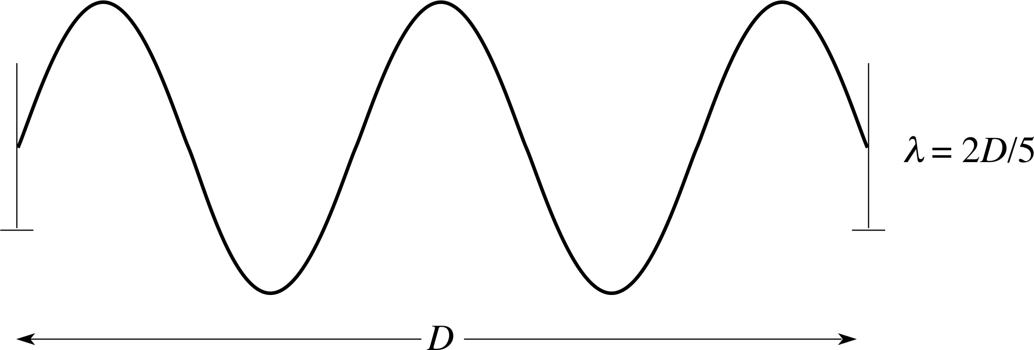
Figure 11 See Answer E4.
Answer E4
The spatial wavefunction that has five half wavelengths within the box is shown in Figure 11. The wavelength is given by: D = 5λ/2 and nx = 5.
(a) The expression for this spatial wavefunction is
ψ5(x) = A sin(5πx D).
(b) Since λ = 2D/5 and p = h/λ it is tempting to say that px = 5h/(2D). But more caution is needed. Such certainty would conflict with the uncertainty principle in this case. In fact the localization of the particle means that the wavelength is not uniquely determined in this case, as was discussed in the answer to Question T8, but we can say px = ±5h/20.
(c) The energy is entirely kinetic and so:
$E_5 = \dfrac{p^2}{2m} = \dfrac{1}{2m}\left(\dfrac{5h}{2D}\right)^2 = \dfrac{25h^2}{8mD^2}$
Alternatively, the energy level for n = 5 is
$E_5 = \dfrac{n^2h^2}{8mD^2} = \dfrac{25h^2}{8mD^2}$
(Reread Subsections 4.1 and 4.2 if you had difficulty with this question.)
Question E5 (A8)
A particle confined to be within a cube of side D is in a stationary state with a spatial wavefunction:
$\psi_{n_x,n_y,n_z}(x,\,y,\,z) = A_n\sin\left(\dfrac{n_x\pi x}{D}\right)\sin\left(\dfrac{n_y\pi y}{D}\right)\sin\left(\dfrac{n_z\pi z}{D}\right)$
and with energy:
$E_{n_x,n_y,n_z} = \dfrac{h^2}{8mD^2}(n_x^2+n_y^2+n_z^2)$
(a) What does it mean to say that an energy level is degenerate?
(b) The energy level 7h2/(4mD2) is degenerate. Determine the order of degeneracy and give expressions for the corresponding wavefunctions.
Answer E5
(a) An energy level is degenerate if more than one wavefunction corresponds to the energy value.
(b) The energy value 7h2/4mD2, i.e. 14h2/8mD2 implies that (nx2 + ny2 + nz2) = 14.
One set of quantum numbers that satisfies this condition is:
(1) nx = 1, ny = 2, nz = 3.
The other combinations that also give the same energy are:
(2) nx = 1, ny = 3, nz = 2;
(3) nx = 2, ny = 1, nz = 3;
(4) nx = 2, ny = 3, nz = 1;
(5) nx = 3, ny = 1, nz = 2;
(6) nx = 3, ny = 2, nz = 1.
There are six combinations corresponding to six different wavefunctions, so the order of degeneracy is six. The six corresponding spatial wavefunctions are:
(1) $\psi_{1,2,3}(x,\,y,\,z) = A\sin\left(\dfrac{\pi x}{D}\right)\sin\left(\dfrac{2\pi y}{D}\right)\sin\left(\dfrac{3\pi z}{D}\right)$
(2) $\psi_{1,3,2}(x,\,y,\,z) = A\sin\left(\dfrac{\pi x}{D}\right)\sin\left(\dfrac{3\pi y}{D}\right)\sin\left(\dfrac{2\pi z}{D}\right)$
(3) $\psi_{2,1,3}(x,\,y,\,z) = A\sin\left(\dfrac{2\pi x}{D}\right)\sin\left(\dfrac{\pi y}{D}\right)\sin\left(\dfrac{3\pi z}{D}\right)$
(4) $\psi_{2,3,1}(x,\,y,\,z) = A\sin\left(\dfrac{2\pi x}{D}\right)\sin\left(\dfrac{3\pi y}{D}\right)\sin\left(\dfrac{\pi z}{D}\right)$
(5) $\psi_{3,1,2}(x,\,y,\,z) = A\sin\left(\dfrac{3\pi x}{D}\right)\sin\left(\dfrac{\pi y}{D}\right)\sin\left(\dfrac{2\pi z}{D}\right)$
(6) $\psi_{3,2,1}(x,\,y,\,z) = A\sin\left(\dfrac{3\pi x}{D}\right)\sin\left(\dfrac{2\pi y}{D}\right)\sin\left(\dfrac{\pi z}{D}\right)$
(Reread Subsections 5.1, and 5.2 if you have difficulty with this question.)
Study comment This is the final Exit test question. When you have completed the Exit test go back and try the Subsection 1.2Fast track questions if you have not already done so.
If you have completed both the Fast track questions and the Exit test, then you have finished the module and may leave it here.
Study comment Having seen the Fast track questions you may feel that it would be wiser to follow the normal route through the module and to proceed directly to the following Ready to study? Subsection.
Alternatively, you may still be sufficiently comfortable with the material covered by the module to proceed directly to the Section 6Closing items.