PHYS 11.3: Schrödinger’s model of the hydrogen atom |
PPLATO @ | |||||
PPLATO / FLAP (Flexible Learning Approach To Physics) |
||||||
|
1 Opening items
1.1 Module introduction
The hydrogen atom is the simplest atom. It has only one electron and the nucleus is a proton. It is therefore not surprising that it has been the test–bed for new theories. In this module, we will look at the attempts that have been made to understand the structure of the hydrogen atom – a structure that leads to a typical line spectrum.
Nineteenth century physicists, starting with Balmer, had found simple formulae that gave the wavelengths of the observed spectral lines from hydrogen. This was before the discovery of the electron, so no theory could be put forward to explain the simple formulae. However, even after the discovery of the nuclear atom by Rutherford in 1912, the classical physics of the nineteenth century, when applied to the electron in the atom, could not account for the hydrogen spectrum at all. Indeed, the theory predicts that an electron in orbit about the proton will continuously emit electromagnetic radiation. The loss of energy by the electron will cause it to spiral in towards the proton and eventually crash into it within a tiny fraction of a second. Classical theory, therefore, not only fails to predict the characteristic line spectra, it suggests that the atom is inherently unstable!
The arrival of the quantum theory at the beginning of the twentieth century offered a new approach. Initially, the theory was applied to radiation. Radiation of frequency f transfers its energy in quanta of amount hf. Application to the hydrogen atom was first tried by Niels Bohr in 1913. He started by looking at the electron in a circular orbit about the proton and derived an expression for the corresponding energy levels. Transitions by the electron between these levels, according to Bohr’s quantum theory of the atom, correctly predicted the wavelengths of the spectral lines. We will look at the elements of Bohr’s argument in Subsection 2.1.
This theory represented a significant advance on classical physics. It used an amalgam of classical physics and what has become known as the ‘old quantum theory’. However, as frequently happens, the success did not survive closer examination and the advances in knowledge after Bohr’s work. Attempts to extend the simple circular orbit model and to introduce refinements required by Einstein’s theory of relativity led to inconsistencies between predictions and experimental observations.
The situation was changed again when it was discovered that the electron had wave–like properties. This had been suggested by Louis de Broglie and was confirmed by the observation of electron diffraction. This idea was incorporated in to the ‘new quantum theory’ which is expressed by the Schrödinger wave equation. This non–classical wave behaviour completely undermines the Bohr approach – the electron may not be considered classically at all, not even ‘semi-classically’.
In Section 2 we review the Bohr model for hydrogen and the early ideas of de Broglie waves as applied to the Bohr model. Section 3 introduces the Schrödinger model, setting up the Schrödinger equation for atomic hydrogen, describing its solutions and the quantum numbers which arise from these solutions. Finally a comparison between the Schrödinger model and the Bohr model is made.
Study comment Having read the introduction you may feel that you are already familiar with the material covered by this module and that you do not need to study it. If so, try the following Fast track questions. If not, proceed directly to the Subsection 1.3Ready to study? Subsection.
1.2 Fast track questions
Study comment Can you answer the following Fast track questions? If you answer the questions successfully you need only glance through the module before looking at the Subsection 4.1Module summary and the Subsection 4.2Achievements. If you are sure that you can meet each of these achievements, try the Subsection 4.3Exit test. If you have difficulty with only one or two of the questions you should follow the guidance given in the answers and read the relevant parts of the module. However, if you have difficulty with more than two of the Exit questions you are strongly advised to study the whole module.
Question F1
In the Bohr model of the hydrogen atom, the electron moves in a circular orbit about the proton. What is the angular momentum of the electron that is in the state with n = 5?
Answer F1
In the Bohr model, the quantum number n gives the orbital angular momentum of the electron in its circular orbit in units of h/2π. The angular momentum is, therefore, 5h/2π.
Question F2
Sketch the de Broglie standing wave for the n = 5 state in Question F1.
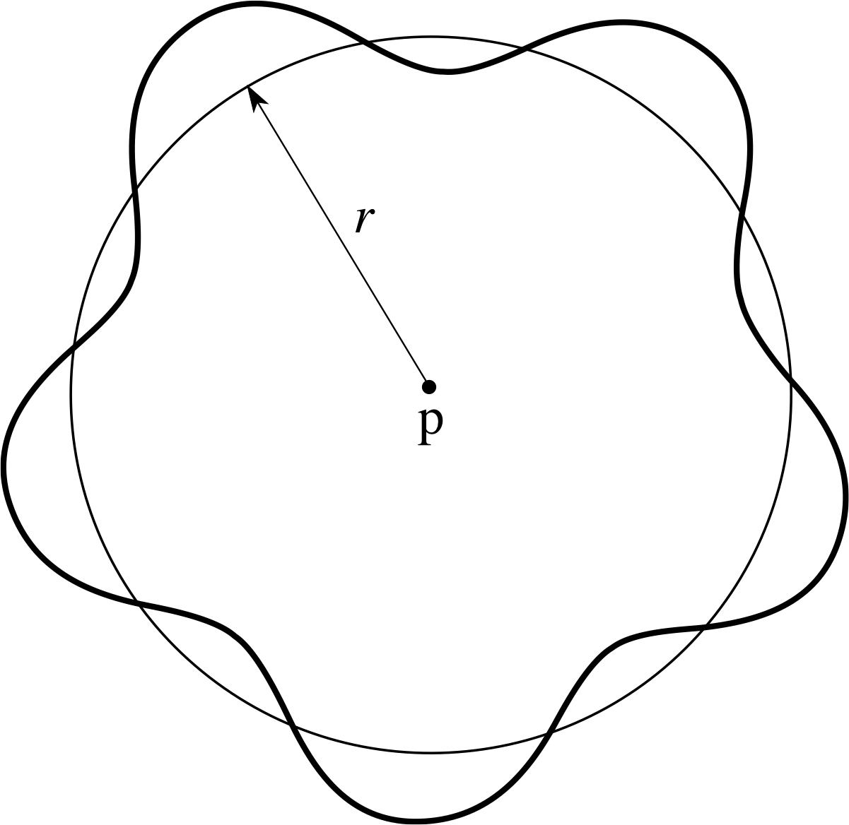
Figure 3 A stationary electron wave ‘orbiting’ a proton. Note that the circumference of the circle contains a whole number of wavelengths of the wave.
Answer F2
The radius of the Bohr orbit with n = 5 is 52a0, where a0 is the Bohr radius. In the stationary state, the orbit holds 5 wavelengths.
It appears, therefore, as sketched in Figure 3.
Question F3
The Schrödinger wavefunction for the electron in a hydrogen atom may be written: ψn l (r) Yl m(θ, ϕ), where (r, θ, ϕ) are spherical polar coordinates.
(a) Show on Cartesian axes how r, θ and ϕ are defined.
(b) Write down the usual symbols for the three quantum numbers of the electron state.
(c) State how two of the quantum numbers are related to the angular momentum of the electron.
Answer F3
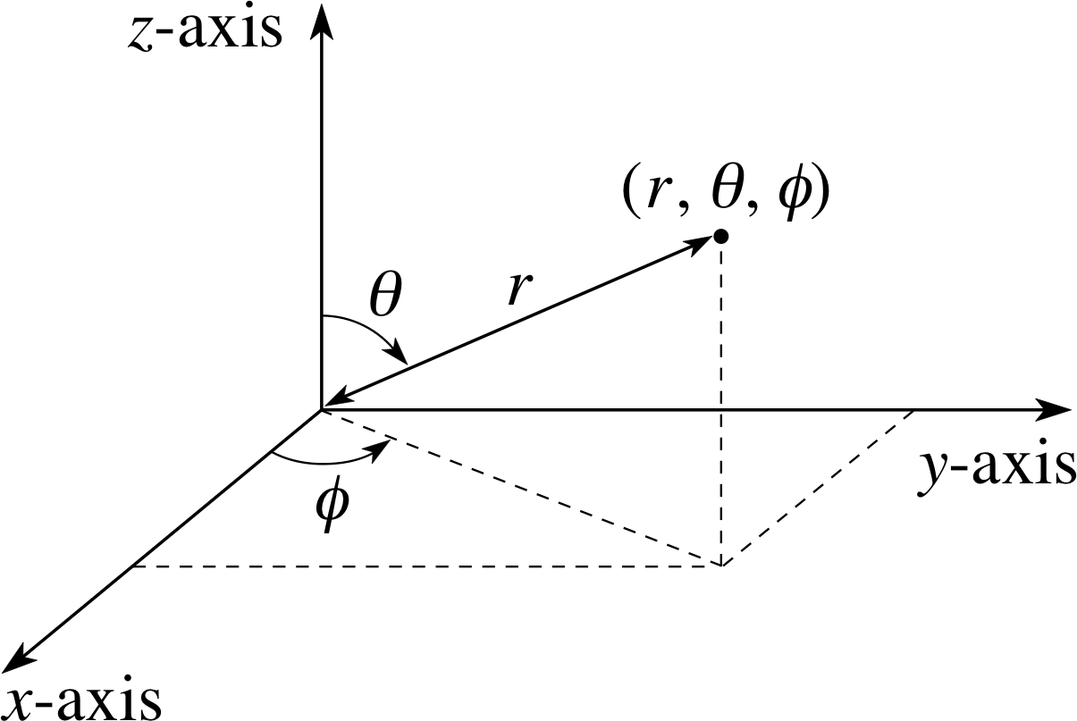
Figure 6 Specifying a point using spherical polar coordinates r, θ, ϕ.
(a) The coordinates r, θ and ϕ are defined as shown in Figure 6.
(b) The three quantum numbers of the electron state are n, l and m.
(c) The quantum numbers related to the angular momentum of the electron are l and m. The z–component of angular momentum is m, where is h/2π.
The magnitude of the orbital angular momentum is $\sqrt{l(l+1)\os}\hbar$.
Question F4
(a) What is the degeneracy of the 3d electron state?
(b) If an electron in this state makes a transition to a 2p state, how much energy is released?
Answer F4
(a) The 3d state has the quantum numbers n = 3, l = 2. The degeneracy of an l–state is 2l + 1, so the 3d state is 5-fold degenerate.
(b) The energy of an electron in a hydrogen atom is given by: En = −13.6 eV/n2. The 3d state therefore has energy −1.51 eV and the energy of the 2p state is −3.40 eV.
The transition from one state to the other therefore releases about 1.89 eV.
1.3 Ready to study?
Study comment In order to study this module, you will need to be familiar with the following physics terms: angular momentum, centripetal force, Coulomb force, de Broglie wavelength, electron, electronvolt (eV), kinetic_energykinetic, potential_energypotential and energytotal energy, Newton’s second law of motion, Planck’s constant h, the Planck–Einstein formula, probabilityprobability wave, proton, quanta, the Schrödinger equation, spectral lines, stationary wave. The mathematical requirements are a knowledge of differentiation, integration, and complex numbers. If you are uncertain about any of these terms, then you can review them now by referring to the Glossary, which will also indicate where in FLAP they are developed. The following Ready to study questions will allow you to establish whether you need to review some of the topics before embarking on this module.
Question R1
If an electron were in a circular orbit of radius 5.0 × 10⁻¹⁰ m with a speed of 2.0 × 10⁷ m s−1, what would be the magnitude of its angular momentum, (a) in SI units, and (b) in units of h?
[Take me = 9.1 × 10⁻³¹ kg and h = 6.6 × 10⁻³⁴ J s.]
Answer R1
The magnitude of the momentum is 9.1 × 10−31 kg × 2.0 × 107 m s−1 = 1.82 × 10⁻²³ kg m s−1.
Therefore the magnitude of the orbital angular momentum L is equal to
1.82 × 10⁻²³ kg m s−1 × 5 × 10−10 m = 9.1 × 10⁻³³ kg m2 s−1 = 9.1 × 10⁻³³ J s
In units of h $L = \dfrac{9.1\times10^{-33}}{6.6\times10^{-34}}\,h \approx 14\,h$
Question R2
An electron undergoes a transition from a state with energy −5 eV to a state with energy −15 eV. What is the frequency of the quantum of electro–magnetic radiation that is emitted?
Answer R2
Energy change = energy before transition − energy after = −5 eV − (−15 eV) = +10 eV
This energy is emitted as a quantum of electromagnetic radiation whose frequency, f, is given by the Planck–Einstein formula: ∆E = hf.
Therefore the frequency is:
$f = \rm \dfrac{10\times1.6\times10^{-19}\,J}{6.6\times10^{-34}\,s} = 2.4\times10^{15}\,Hz$
Question R3
Write down the time–independent Schrödinger equation of an electron subject to a potential energy field U (x) in one dimension. What interpretation is given to the solution ψ (x)?
Answer R3
The time–independent Schrödinger equation in one dimension may be written:
$-\dfrac{\hbar^2}{2m\os}\dfrac{d^2\psi(x)}{dx^2} + U(x)\psi(x) = E_{\rm tot}\psi(x)$
where Etot is the total energy of the electron.
The eigenfunctionenergy eigenfunction ψ (x) is the spatial part of a stationary_statestationary state wavefunction.
It is also the probability density function for the electron. That is, the probability of finding the electron in the small region from x to x + ∆x is given by | ψ (x) |2 ∆x.
2 The early quantum models for hydrogen
2.1 Review of the Bohr model
The Bohr model is a mixture of classical physics and quantum physics. i It is based on four postulates.
Postulate 1 The electron in the atom moves in a circular orbit centred on its nucleus which is a proton. Its motion in the orbit is governed by the Coulomb electric force between the negatively charged electron and the positively charged proton.
Postulate 2 The motion of the electron is described by Newton’s laws of motion in all but one respect – the magnitude L of the electron’s angular momentum is quantized in units of Planck’s constant divided by 2π. So:
$L = n\left(\dfrac{h}{2\pi}\right)$(1)
where the number n (known as the Bohr quantum number) can have the integer values n = 1 or 2 or 3, etc. Postulate 2 includes an acception of classical mechanics except for one new feature, which is a ‘quantization’ hypothesis concerning the angular momentum of the electron in its orbit.
The angular momentum is the moment of linear momentum. For the circular orbit of radius r in which the electron has a constant speed υ, the magnitude of the angular momentum L = r × meυ = meυr. In classical mechanics any value of L would be allowed depending on the radius of the orbit. This latter result was abandoned by Bohr.
In this case the radial acceleration (centripetal acceleration) has a magnitude υ2/r with the radial force (centripetal force) towards the centre of magnitude meυ2/r. This centripetal force is provided by the attractive Coulomb force and is of magnitude
$F = \dfrac{1}{4\pi\varepsilon_0}\dfrac{e^2}{r^2}$
So, equating these magnitudes we have:
$m_{\rm e}\dfrac{\upsilon^2}{r} = \dfrac{1}{4\pi\varepsilon_0}\dfrac{e^2}{r^2}$(2)
This may be rearranged to give:
$m_{\rm e}^2\upsilon^2r^2\left(=L^2\right) = \dfrac{m_{\rm e}e^2}{4\pi\varepsilon_0}r$(3)
The Bohr quantization condition (Equation 1) then implies a restriction on the orbits, so that the allowed orbits are given by
$\left(n\dfrac{h}{2\pi}\right)^2 = \dfrac{m_{\rm e}e^2}{4\pi\varepsilon_0}r$ where n = 1, 2, 3, ...
i.e.$r = n^2 \dfrac{\varepsilon_0^2 h^2}{\pi m_{\rm e} e^2} \equiv n^2a_0$(4)
The constant ε0h2/(πmee2) has been denoted a0. It is the radius of the smallest orbit (for which n = 1) and is usually called the Bohr radius, a0 and has the value 0.53 × 10⁻¹⁰ m. Look up the values of the physical constants in Equation 4 and verify this value.
We have applied the Bohr quantization and seen that it restricts the radii of permitted orbits. However, this is not a great enough departure from classical physics to explain the stability of the atom, since classical electromagnetism would still lead to continuous emission of radiation from the orbiting electron and the consequent collapse of the atom. We also need:
Postulate 3 An electron in a Bohr orbit does not continuously radiate electromagnetic radiation. Its energy is therefore constant. The orbit is referred to as a stationary orbit.
To account for the observed spectrum we need:
Postulate 4 Electromagnetic radiation is only emitted when the electron changes from one orbit to another of a lower total energy. (The electron is said to undergo a transition.) In such a case, the energy lost, ∆E, is emitted as one quantum of radiation of frequency f as given by the Planck–Einstein formula:
∆E = hf(5)
It is this last condition which predicts that the frequencies of radiation emitted from a hydrogen atom have only certain values.
To make this precise, we need to find the energy of an electron in an allowed orbit characterized by a particular value of n. This energy is made up of two parts: the kinetic energy $\frac12 m_{\rm e}\upsilon^2$ and the potential energy, which, for the Coulomb force field, is $-\dfrac{1}{4\pi\varepsilon_0}\dfrac{e^2}{r}$ (the negative sign is needed because the force is one of attraction and the zero of potential energy is taken at r = ∞).
Thus$E = \frac{1}{2}m_{\rm e}\upsilon^2 - \dfrac{1}{4\pi\varepsilon_0}\dfrac{e^2}{r}$
However, from Equation 2,
$m_{\rm e}\dfrac{\upsilon^2}{r} = \dfrac{1}{4\pi\varepsilon_0}\dfrac{e^2}{r^2}$(Eqn 2)
$m_{\rm e}{\upsilon^2} = \dfrac{1}{4\pi\varepsilon_0}\dfrac{e^2}{r}\quad\text{so that}~~E = -\dfrac12\dfrac{1}{4\pi\varepsilon_0}\dfrac{e^2}{r}$ and, using Equation 4,
$r = n^2\dfrac{\varepsilon_0h^2}{\pi m_{\rm e}e^2} \equiv n^2a_0$(Eqn 4)
It follows that the stationary orbit with the quantum number n has energy, En, given by:
$E_n = - \dfrac{m_{\rm e}e^4}{8\varepsilon_0^2h^2}\dfrac{1}{n^2}$(6)
which in units of electronvolts is
$E_n = - \dfrac{\rm 13.6\,eV}{n^2}$(6a)
| quantum number, n |
radius of orbit |
energy/eV |
|---|---|---|
| 1 | a0 | −13.6 |
| 2 | 4 a0 | −3.4 |
| 3 | 9 a0 | −1.5 |
| 4 | 16 a0 | −0.85 |
Thus the orbits and energies of the electron are restricted. The first four are shown in Table 1. The energies listed in Table 1 are negative because they represent bound states with the energy zero taken where the electron is at rest an infinite distance from the proton.
The combination of this result and the Planck–Einstein formula gives the main prediction that may be tested in the laboratory – by observing the frequencies of the spectral lines that hydrogen atoms actually emit.
It is predicted that if an electron in a stationary orbit with quantum number n1 undergoes a transition to a lower energy orbit with quantum number n2, then the loss of energy ∆E = En1 − En2 is emitted as a quantum of radiation with the frequency, fn1→n2, calculated using Equation 5,
∆E = hf(Eqn 5)
With Equation 6, the frequency is:
$f_{n_1\to n_2} = \dfrac{m_{\rm e}e^4}{8\varepsilon_0^2h^3}\left(\dfrac{1}{n_2^2}-\dfrac{1}{n_1^2}\right)$(7)
This is the main prediction of the Bohr model. The spectra observed in the laboratory fit the predictions very closely. For a fuller discussion of this, you should refer to the Bohr model elsewhere in FLAP.
Question T1
An electron in a hydrogen atom has an energy of −0.544 eV. What is the magnitude of the angular momentum of the electron according to the Bohr model? How much energy will be released if the electron makes a transition to the orbit with one unit ($\hbar$) i less angular momentum?
Answer T1
The Bohr model gives, for the energy of the electron in the hydrogen atom, the formula:
$E_n = \dfrac{\rm -13.6\,eV}{n^2}$
where the electron has quantum number n.
Its angular momentum is $nh/(2\pi) = n\hbar$.
Now since 0.544 = 13.6/n2, n = 5 and the electron has an angular momentum of magnitude $5\hbar$. The state with one unit of angular momentum less has n = 4 and energy E4 = −13.6 eV/42 = −0.850 eV. The energy released is −0.544 eV − (−0.850 eV) = 0.306 eV.
We will not extend this discussion any further. We wished to look at the basic form of the model, to mention its successes and highlight its main assumptions. We have seen that the model is a hybrid of classical and quantum physics. The mechanics is that of Newton but with restrictions on the angular momentum magnitudes. The classical theory of radiation emission is suspended in the stationary orbits; emission takes place in single quanta and occurs only as the result of changes of orbit.
In the next subsection, we will examine another fundamental departure from classical physics – the wave–like behaviour of matter – and see how a simplistic application of this new phenomenon gives an insight into why it is that angular momentum might be quantized.
2.2 The wave–like properties of the electron
The hypothesis that matter has wave–like properties and the observation of electron diffraction undermined the Bohr model, which was based on a classical particle view of the electron. In the new situation, the behaviour of the electron in the hydrogen atom will be governed by its wave equation – the Schrödinger equation – and not by classical Newtonian particle laws. We will start to look at this new situation in the next subsection, but first we want to investigate how the new situation gives an insight into the existence of restrictions on the allowed orbits in an atom. In the case of the Bohr model, these were postulated. There was no obvious underlying reason why they should arise.
We will start from the de Broglie relation i between the magnitude of the momentum, p, of an electron and its corresponding wavelength λdB:
λdB = hp(8)
We know that classical waves, such as water waves or electromagnetic waves, are characterized by a wavefunction which describes the wave disturbance at any given position and time. In the case of water waves, the disturbance is the displacement of the water surface from its equilibrium position; in the case of classical electromagnetic waves, the disturbance is the departure of the electric field from its equilibrium value.
In the case of the quantum waves of electrons, the wavefunction, Ψ, is not a measurable physical quantity because the wave is a probability wave. In one dimension, for example, the value of | Ψ (x, t) |21∆x is the probability of finding the electron, say, between x and x + ∆x at time t. However, in other respects, because the function Ψ (x, t) satisfies a sort of wave equation, the properties of classical waves will be similar to the properties of electron probability waves.
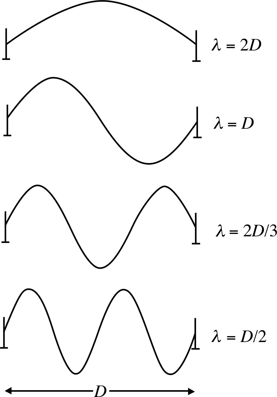
Figure 1 Four of the standing waves that may be set up on a taut, elastic string that is fixed at each end. The diagrams are not to scale, and are only snapshots of the waves, each of which varies with time.
One such property is the existence of standing_wavestanding, or stationary_wavestationary, waves. Consider an elastic string, such as the string of a guitar, which is under tension and fixed at its two ends. The string, if plucked, will oscillate as shown in Figure 1.
We note that the modes of oscillation of the string all have a characteristic feature – the string is oscillating with an integral number of half–wavelengths confined between the fixed ends. In this way, for the string, only a certain set of wavelengths are permitted – those given by D = nλ/2 with n an integer, n = 1, 2, 3, .... This restriction is imposed by the boundary condition: the string is fixed at each end.
Let us now see how this might relate to the Bohr model if we take account of the wave–like nature of the electron. This discussion will also be semi–classical since we will not consider the Schrödinger equation but only a simple wave picture.
We will start from the idea of a circular orbit with radius r. We will suppose that the electron ‘orbits’ the proton, but instead of its path being described by a definite classical trajectory as shown in Figure 2a, we will suppose that it is represented as a wave travelling around the proton. Such a wave might be ‘pictured’ as in Figure 2b.
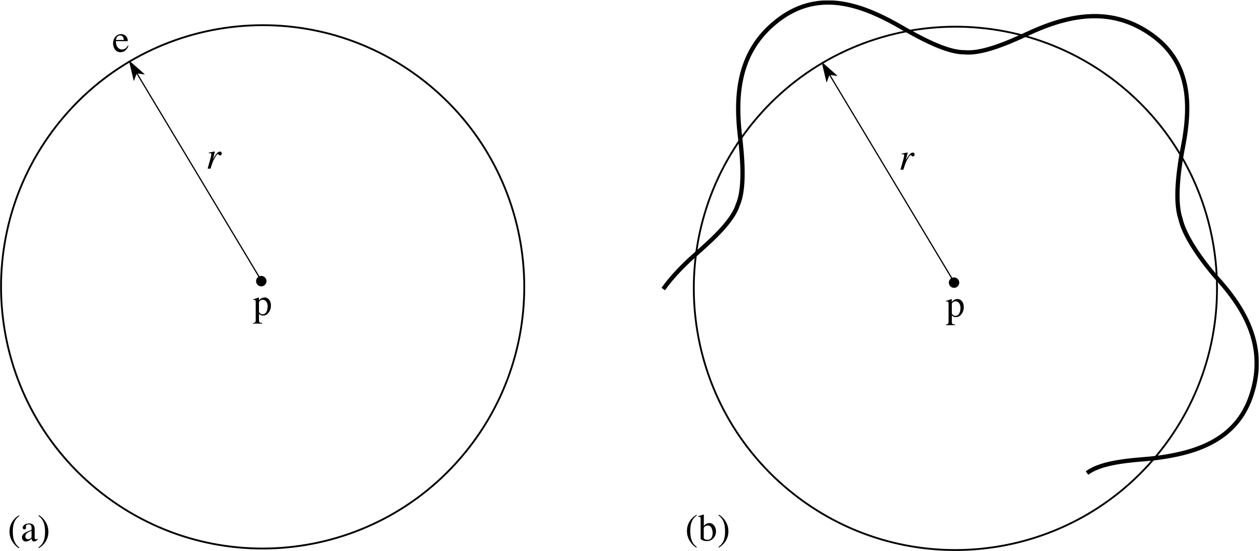
Figure 2 (a) A classical circular orbit of an electron about a proton. (b) An electron wave pictured ‘orbiting’ the proton. Note that the bold line is not the trajectory of the electron. It is part of a wave with its amplitude measured from the circle shown.
We might now ask if there are any restrictions on such waves if they are to be stable features of the electron in the hydrogen atom – for this is what stationary orbits are meant to represent. Since we want our wave to persist, rather than cancelling itself out by interference, it seems sensible to require that a whole number of its wavelengths should fit around the orbit, as shown in Figure 3. This boundary condition would make it a stationary wave, but it also implies a relationship between the wavelength and the orbital radius.
According to Bohr’s model, an electron in an orbit of radius r has a momentum magnitude p = [mee2/(4πε0r)]1/2. So its de Broglie wavelength λdB = h/p is determined by r. Consequently, only certain orbital radii will meet the requirement that the circumference of the orbit must contain an integer number of whole de Broglie wavelengths:
2πr = nλdB n = 1, 2, 3, ...(9)
Figure 3 A stationary electron wave ‘orbiting’ a proton. Note that the circumference of the circle contains a whole number of wavelengths of the wave.
Combining Equations 8 and 9, this restriction becomes:
$2\pi r = n\dfrac hp$
which may be written:
$pr = n\dfrac{h}{2\pi}$(10)
If we now remember that classical angular momentum, L, is the moment of linear momentum, then the left–hand side of Equation 10 is the magnitude of the angular momentum of an electron of momentum p in a circular orbit of radius r. Thus Equation 10 is the same as Equation 1,
$L = n\left(\dfrac{h}{2\pi}\right)$(Eqn 1)
which was a postulate of the Bohr theory.
So we see that the wave picture of the electron leads to a postulate of the Bohr model. However the treatment here is still semi-classical. We now turn to the full wave model by considering the Schrödinger equation for the electron in the hydrogen atom.
3 The Schrödinger model for hydrogen
Although the Bohr model hypothesis for the quantization of angular momentum can be justified in terms of electron wave ideas, the Bohr model remains profoundly unsatisfactory as a wave model for the atom.
A full quantum wave model for the atom must incorporate a wave equation as its basis, in the same way that a wave equation is used to model waves on a string, or water waves or electromagnetic waves or indeed any of the waves of classical physics. i What is required is a wave equation for the de Broglie waves, and for the hydrogen atom we can anticipate that standing wave solutions should emerge from this equation once the physical boundary conditions are imposed. The Schrödinger equation is the key development here, it is the wave equation for de Broglie waves and its solution lies at the heart of quantum mechanics.
3.1 The potential energy function and the Schrödinger equation
Study comment In quantum mechanics, the wavefunction Ψ (x, t) describing a one–dimensional stationary state, of fixed energy E, is given by
${\it\Psi}(x,\,t) = \psi(x)\exp\left(-i\dfrac{E}{\hbar}t\right)$
Since we will only be concerned with such constant energy states we may take the time–dependent factor $\exp\left(-i\dfrac{E}{\hbar}t\right)$ for granted, and concentrate on the determination of the energy E and the corresponding spatial part of the wavefunction ψ (x). In the case of linear motion, both of these quantities are obtained by solving the time–independent Schrödinger equation, which is introduced elsewhere in FLAP.
The time–independent Schrödinger equation for a particle of mass m moving in one–dimension can be written as:
$-\dfrac{\hbar^2}{2m\os}\dfrac{d^2\psi(x)}{dx^2} + U(x)\psi(x) = E\psi(x)$(11)
Here U (x) is the potential energy function, the first term is associated with the kinetic energy and E is the total energy. These associations can be expressed in the more formal language of quantum mechanics in terms of operators and eigenvalue equations. i
An operator is an instruction to carry out some operation on a function. The differential operator $-\dfrac{\hbar^2}{2m\os}\dfrac{d^2\psi(x)}{dx^2}$ operates on the function ψ (x) by taking the second derivative of the function with respect to x and then multiplying the result by $-\dfrac{\hbar^2}{2m}$. The result of this operation is to regenerate the same function ψ (x) with a numerical multiplier, in this case the kinetic energy Ekin. We write this as
$-\dfrac{\hbar^2}{2m\os}\dfrac{d^2\psi(x)}{dx^2} = E_{\rm kin}\psi(x)$(12)
This is an example of an eigenvalue equation in which an operator acts on a function, called an eigenfunction, to produce the same function with a numerical multiplier, which is called an eigenvalue of the operator.
This is illustrated as:
$\fbox{operator}~~~\raise 7pt {\underrightarrow{{\text{acting on}}}}~~~\fbox{eigenfunction} = \fbox{eigenvalue} \times \fbox{eigenfunction}$
In quantum mechanics each physical observable (such as kinetic energy, total energy, momentum, or angular momentum) has an associated operator which forms part of an eigenvalue equation, with the allowed values of the observables being given by the eigenvalues. If an eigenfunction representing a state of the system is simultaneously an eigenfunction of several such operators then the associated eigenvalues of these operators represent the outcomes of appropriate measurements carried out on the system, when in this state.
Equation 11 itself is an eigenvalue equation. We can associate the total energy operator, or Hamiltonian operator
$\bar{\rm H} = -\dfrac{\hbar^2}{2m\os}\dfrac{d2^\psi(x)}{dx^2} + U(x)$(13) i
as the sum of the operators for kinetic and potential energy. The eigenvalue is the total energy E. Equation 11 can then be written as
$\hat{\rm H}\psi(x) = E\psi(x)$(14)
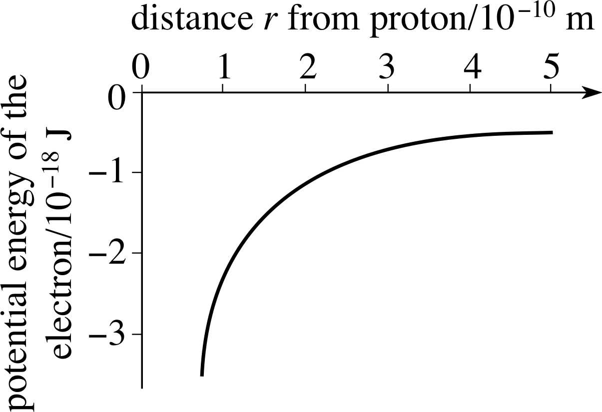
Figure 4 The form of the potential energy of the electron as a function of its distance, r, from the proton.
For the hydrogen atom the problem is three–dimensional and the energy eigenfunctions are ψ (x, y, z). The potential energy function U (x) is the Coulomb potential energy, which depends only on the distance of separation $r = \sqrt{\smash[b]{x^2 + y^2 + z^2}}$ between the electron and the nucleus (proton), as shown in Figure 4.
$U(r) = -\dfrac{e^2}{4\pi\varepsilon_0r}$
The kinetic energy operator for three–dimensional motion can be obtained by a generalization of the one–dimensional case. In classical physics we can write the kinetic energy for three–dimensional motion at speed υ as:
$E_{\rm kin} = \frac12m\upsilon^2 = \frac12m(\upsilon_x^2 + \upsilon_y^2 + \upsilon_z^2) = \frac12m\upsilon_x^2 + \frac12m\upsilon_y^2 + \frac12m\upsilon_z^2$
In quantum mechanics, for three–dimensional motion we extend Equation 12,
$-\dfrac{\hbar^2}{2m\os}\dfrac{d^2\psi(x)}{dx^2} = E_{\rm kin}\psi(x)$(Eqn 12)
by writing:
$-\dfrac{\hbar^2}{2m\os}\left[\dfrac{\partial^2}{\partial x^2}+\dfrac{\partial^2}{\partial y^2}+\dfrac{\partial^2}{\partial z^2}\right]\psi(x,\,y,\,z) = E_{\rm kin}\psi(x,\,y,\,z)$(15) i
We need to use partial derivatives here since we now have three separate spatial variables. The Hamiltonian operator becomes:
$-\dfrac{\hbar^2}{2m\os}\left[\dfrac{\partial^2}{\partial x^2}+\dfrac{\partial^2}{\partial y^2}+\dfrac{\partial^2}{\partial z^2}\right] - \dfrac{e^2}{4\pi\varepsilon_0r}$(16)
and the eigenfunctions and energy eigenvalues are then found by solving the three–dimensional time–independent Schrödinger equation:
$-\dfrac{\hbar^2}{2m\os}\left[\dfrac{\partial^2}{\partial x^2}+\dfrac{\partial^2}{\partial y^2}+\dfrac{\partial^2}{\partial z^2}\right]\psi(x,\,y,\,z) - \dfrac{e^2}{4\pi\varepsilon_0r}\psi(x,\,y,\,z) = E\psi(x,\,y,\,z)$(17) i
3.2 Qualitative solutions for wavefunctions – the quantum numbers
We will not discuss the mathematical details of the solution of Equation 17. However, we will look at some of its general features that give clues to the relationship between Schrödinger’s quantum–mechanical model and the earlier models of the hydrogen atom.
The first feature relates to the particular nature of the Coulomb potential energy. We note that the potential energy depends only on the distance from the origin (where the proton is located). It does not depend on the orientation of the direction from the proton to the electron.
Figure 6 Alternatively, the point shown in Figure 5 may be specified using spherical polar coordinates r, θ, ϕ.
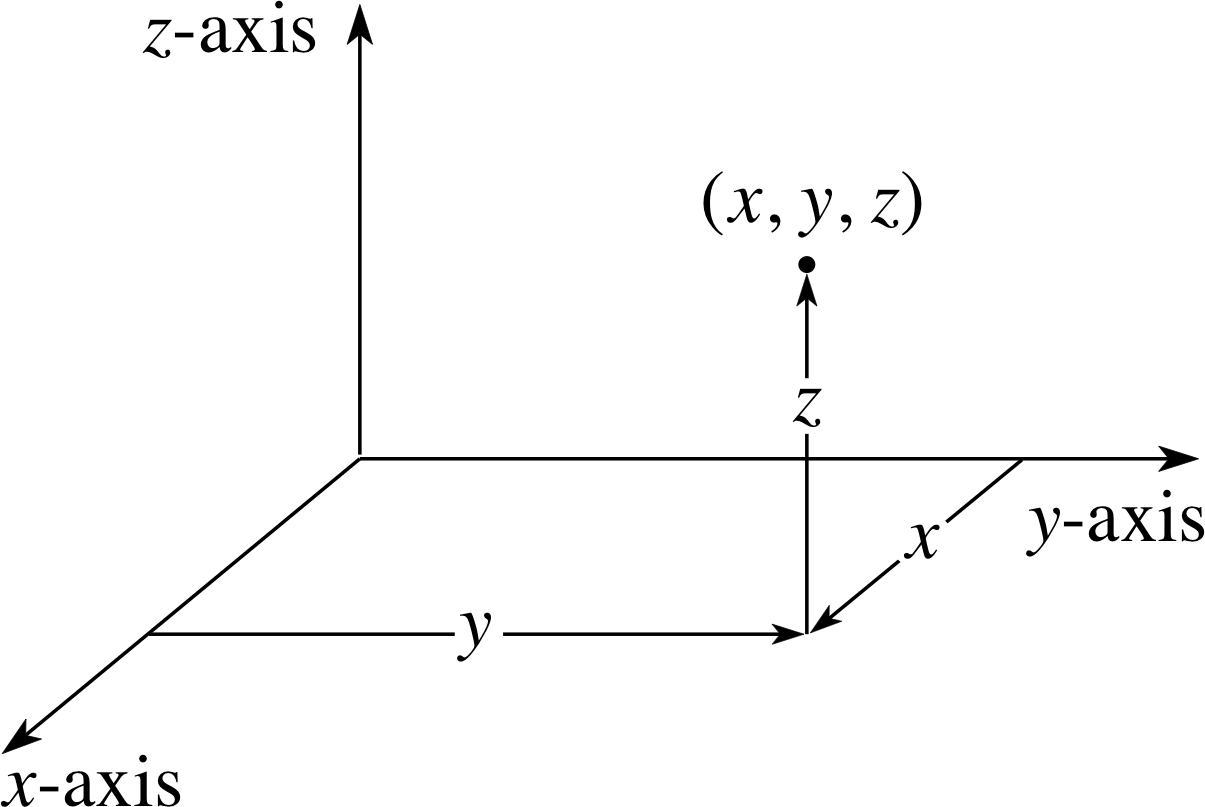
Figure 5 The position of a point in Cartesian coordinates.
With a potential of this type, it is convenient to use not the Cartesian coordinates (x, y, z) of Figure 5, but spherical polar coordinates (r, θ, ϕ) as shown in Figure 6. Then the Coulomb potential energy depends only on the one coordinate r, and not at all on the angular coordinates θ and ϕ shown in Figure 6.
Question T2
With reference to Figure 6, what value of θ gives points on (a) the positive z–axis and (b) the negative z–axis? What are the spherical polar coordinates for the points whose Cartesian coordinates are (i) (2, 10, 10) and (ii) (1, 11, 10)?
Answer T2
Figure 6 Specifying a point using spherical polar coordinates r, θ, ϕ.
(a) The values on the positive z–axis correspond to θ = 0.
(b) The values on the negative z–axis correspond to θ = π (i.e. 180°).
Looking at Figure 6, points in the x–y plane correspond to values of θ = π /2 (i.e. 90°).
(i) Points on the x–axis have values of ϕ = 0. The point (2, 0, 0) is two units away from the origin; so the Cartesian coordinates (2, 0, 0) have the (r, θ, ϕ) equivalent of (2, π/2, 0).
(ii) The point (1, 1, 0) is also in the x–y plane, but with ϕ = π/4 (i.e. 45°). Its distance from the origin is given by Pythagoras’ theorem to be $\sqrt{2\os}$.
So the Cartesian coordinates (1, 1, 0) have the (r, θ, ϕ) equivalent of ($\sqrt{2\os}$, π/2, π/4).
(There is an algebraic formula relating x, y, z to r, θ, ϕ but it is not necessary for our purposes to use it.)
Our task then, is to determine the spatial wavefunctions in terms of these new coordinates: ψ (r, θ, ϕ). When this is done, it turns out that the solutions may be factorized into two parts, ψ (r, θ, ϕ) = R (r) Y (θ, ϕ), and the differential equation, Equation 17,
$-\dfrac{\hbar^2}{2m\os}\left[\dfrac{\partial^2}{\partial x^2}+\dfrac{\partial^2}{\partial y^2}+\dfrac{\partial^2}{\partial z^2}\right]\psi(x,\,y,\,z) - \dfrac{e^2}{4\pi\varepsilon_0r}\psi(x,\,y,\,z) = E\psi(x,\,y,\,z)$(Eqn 17)
separates into two equations, one for the radial part R (r) and one for the angular part, Y (θ, ϕ). This separation is possible because the potential does not depend on θ and ϕ, but only on r. The angular part Y (θ, ϕ) depends on the angular momentum of the electron, and is connected with the angular momentum postulate of Bohr. We will come back to this in a moment. Only the radial part of the wavefunction R (r) depends on the form of the potential energy function.
It is a standard property of eigenvalue equations, such as Equation 17, that the behaviour of the eigenfunctions depends crucially on the boundary conditions that are applied, as we saw in the discussion of the vibrating string in Subsection 2.2. These can only be satisfied for certain special values of the eigenvalues. (For the vibrating spring these correspond to the standing wave frequencies.)
How does this feature apply to the hydrogen atom? The wavefunction must define the probability distribution for the electron in a bound state with the proton. A bound state is one in which the probability that the electron will escape from the attraction of the proton is zero. This means that R (r) must tend to zero as r becomes very large. The special values of the energy that are selected by this condition are a discrete set that may be labelled by the positive integer n, which is called the principal quantum number, and the energy values are, amazingly, exactly the same as Bohr obtained:
$E_n = - \dfrac{m_{\rm e}e^4}{8\varepsilon_0^2h^2}\dfrac{1}{n^2}$(Eqn 6)
The angular part of Equation 17 may be written as
$\hat{\rm L^2}Y(\theta,\,\phi) = l(l +1)\hbar^2Y(\theta,\,\phi)$(18)
where $\hat{\rm L^2}$ is a complicated differential operator involving r, θ and ϕ, which represents the square of the angular momentum of the electron.
The angular wavefunction Y (θ, ϕ), like the radial function, only has acceptable solutions if the eigenvalue $l(l + 1)\hbar^2$ on the right–hand side of Equation 18 takes on certain values; in this case, these are the values obtained by taking l = 0, 1, 2, 3, ..., n − 1, in other words, l must be a non–negative integer smaller than n. Since $\hat{\rm L^2}$ is the operator representing the square of the angular momentum, the eigenvalue $l(l + 1)\hbar^2$ must take on the possible values of the square of the angular momentum L2, and l is usually called the (orbital) angular momentum quantum number:
So$L^2 = l(l + 1)\hbar^2$(19)
However, this is not the whole story. Angular momentum is a vector quantity, and has three Cartesian components Lx, Ly, Lz, which are also represented in quantum mechanics by differential operators. There are too many complications for us to describe the situation in full, but it will be enough to know that the angular wavefunctions Y (θ, ϕ) may also be eigenfunctions of $\hat{L}_z$, which is the operator for Lz, the component of the angular momentum along the z–axis.
$\hat{L}_zY(\theta,\,\phi) = m_l\hbar Y(\theta,\,\phi)$(20)
so$L_z = m_l\hbar$(21)
where ml is an integer, which may only take on the values −l, −l + 1, −l + 2, ... −1, 0, 1, ... l − 1, l; hence there are 2l + 1 possible solutions of Equation 20 for any given l.
The integer ml is called the (orbital) magnetic quantum number.
Thus any wavefunction for the hydrogen atom is specified by three quantum numbers, n, l, and ml. The angular wavefunction must be labelled by l and m, i.e. as Ylm i the radial wavefunction is labelled by n and l, i.e. as Rnl (r), although for the hydrogen atom the energy depends only on the principal quantum number n, as in Equation 6,
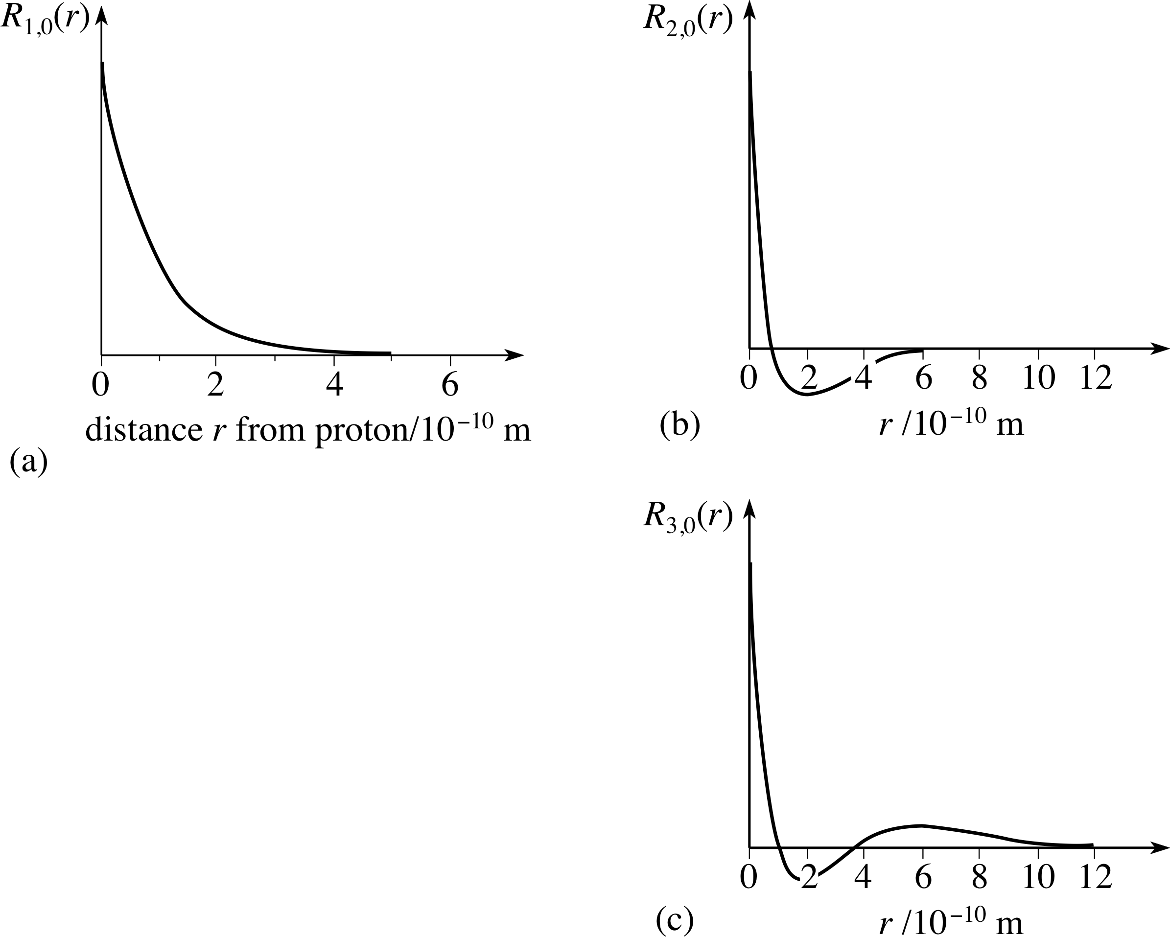
Figure 7 The radial function Rnl (r) for the hydrogen atom for cases with principal quantum number n equal to 1, 2 and 3, and angular momentum quantum number l equal to zero. Note that the function Rn 0 (r) has n − 1 zeros (excluding the limit r → ∞).
$E_n = - \dfrac{m_{\rm e}e^4}{8\varepsilon_0^2h^2}\dfrac{1}{n^2}$(Eqn 6)
Note that this is only true for the hydrogen atom; for any other atom the potential energy will depend on l as well as n, but provided the potential energy does not depend on angle, the angular wavefunctions and the allowable values of the angular momentum will be the same as here.
Figure 7 shows the form of some of the radial wavefunctions for l = 0. The wavefunctions for other values of l are similar, but start from zero at the origin. Equation 19,
$L^2 = l(l + 1)\hbar^2$(19)
shows that the magnitude of the angular momentum of the electron is $\sqrt{l(l+1)\os}\hbar$ which gives a different set of values from the values $\hbar,~2\hbar, \dots$ given by the Bohr theory. The component of angular momentum in the z–direction Lz, however, has the values $-l\hbar$, $-(l-1)\hbar$, $\ldots$ $-\hbar$, 0, $\hbar$, $\ldots$ $(l -1)\hbar$, $l\hbar$.
Question T3
An electron in a hydrogen atom has an angular momentum quantum number l = 2. What is the magnitude of the angular momentum vector? What are the permitted values of the z–components of this angular momentum?
Answer T3
The magnitude of the angular momentum corresponding to quantum number l is $\sqrt{l(l + 1)\os}$.
Therefore the magnitude for l = 2 is $\sqrt{6\os}\hbar$.
The permitted values of the z–component are in general the (2l + 1) values −l, −l + 1, −l + 2, ..., −1, 0, 1, ..., l − 1, l in units of $\hbar$.
The five allowed values for l = 2 are therefore $-2\hbar,~-\hbar,~0,~\hbar,~2\hbar$.
These values show that the angular momentum vector can never entirely be in the z–direction, and that there must always be some non–zero components in the x– and y–directions. However, if we introduce the operators $\hat{L}_x$ and $\hat{L}_y$ that represent the angular momentum components Lx and Ly, we find that they do not have the same eigenfunctions as $\hat{L}_z$:
i.e.$\hat{L}_xY_{l\,m}(\theta,\,\phi) \ne {\rm constant} \times Y_{l\,m}(\theta,\,\phi)$
and$\hat{L}_yY_{l\,m}(\theta,\,\phi) \ne {\rm constant} \times Y_{l\,m}(\theta,\,\phi)$
This means that we cannot simultaneously give exact values to more than one component of angular momentum, although we may know its magnitude.
Question T4
For the electron in Question T3, which has l = 2, sketch a classical vector diagram for the angular momentum vector indicating the smallest angle that the angular momentum can make with the z–axis?
What would be the value of this angle for an electron with l = 100?
Is there a value of l for which the vector points along the z–axis?
Answer T4
The orientation of the angular momentum vector that makes the smallest angle with the z–axis in the case where l = 2 is given in Figure 15. The angle θ2,min is given by:
$\cos\theta_{\rm 2,min} = 2/\sqrt{6\os}$, i.e. $\theta_{\rm 2,min} = 35.3°$
For l = 100, the angle would be given by:
$\cos\theta_{\rm 100,min} = 100/\sqrt{100\times101\os}$, i.e. $\theta_{\rm 100,min} = 5.7°$
Although the angle becomes smaller for larger l, $\sqrt{l(l+1)\os}$ can never be equal to l, so it is not possible for the angular momentum vector to point along either the positive or negative z–direction.
We can summarize this long and complex subsection in the following box and in Table 2, and we suggest that you study it carefully.
- 1
-
Each wavefunction of the bound electron depends on the spherical polar coordinates r, θ, ϕ and the energy eigenfunctions are labelled by three quantum numbers n, l, ml:
ψnlm(r, θ, ϕ)
- 2
-
The Schrödinger equation can be solved separately for the functions depending on the radial coordinate r and on the angular coordinates θ, ϕ. The total energy eigenfunction is the product function:
ψnlm(r, θ, ϕ) = Rnl (r) Ylm(θ, ϕ)
- 3
-
The energy eigenvalue corresponding to ψnlm(r, θ, ϕ) is
$E_n = -\dfrac{m_{\rm e}e^4}{8\varepsilon_0^2h^2}\dfrac{1}{n^2}$
- 4
-
The quantum numbers must obey the restrictions given in Table 2 if the wavefunctions are to be physically meaningful bound state solutions of the Schrödinger equation.
| Name | Allowed values | Role |
|---|---|---|
|
principal quantum number n |
n = 1, 2, 3, ... |
Determines the energy levels of the bound electron |
|
(orbital) angular momentum quantum number l |
l = 0, 1, 2, ... (n − 1) |
Determines the magnitude of the square of the electron’s |
|
(orbital) magnetic quantum number ml |
ml = 0, ±1, ±2, ..., ±l |
Determines the z–component of the electron’s angular |
Figure 8 illustrates the situation for l = 3. For any particular value of ml, the angular momentum vector can be considered to lie anywhere on a cone, the axis of which is the z–axis.
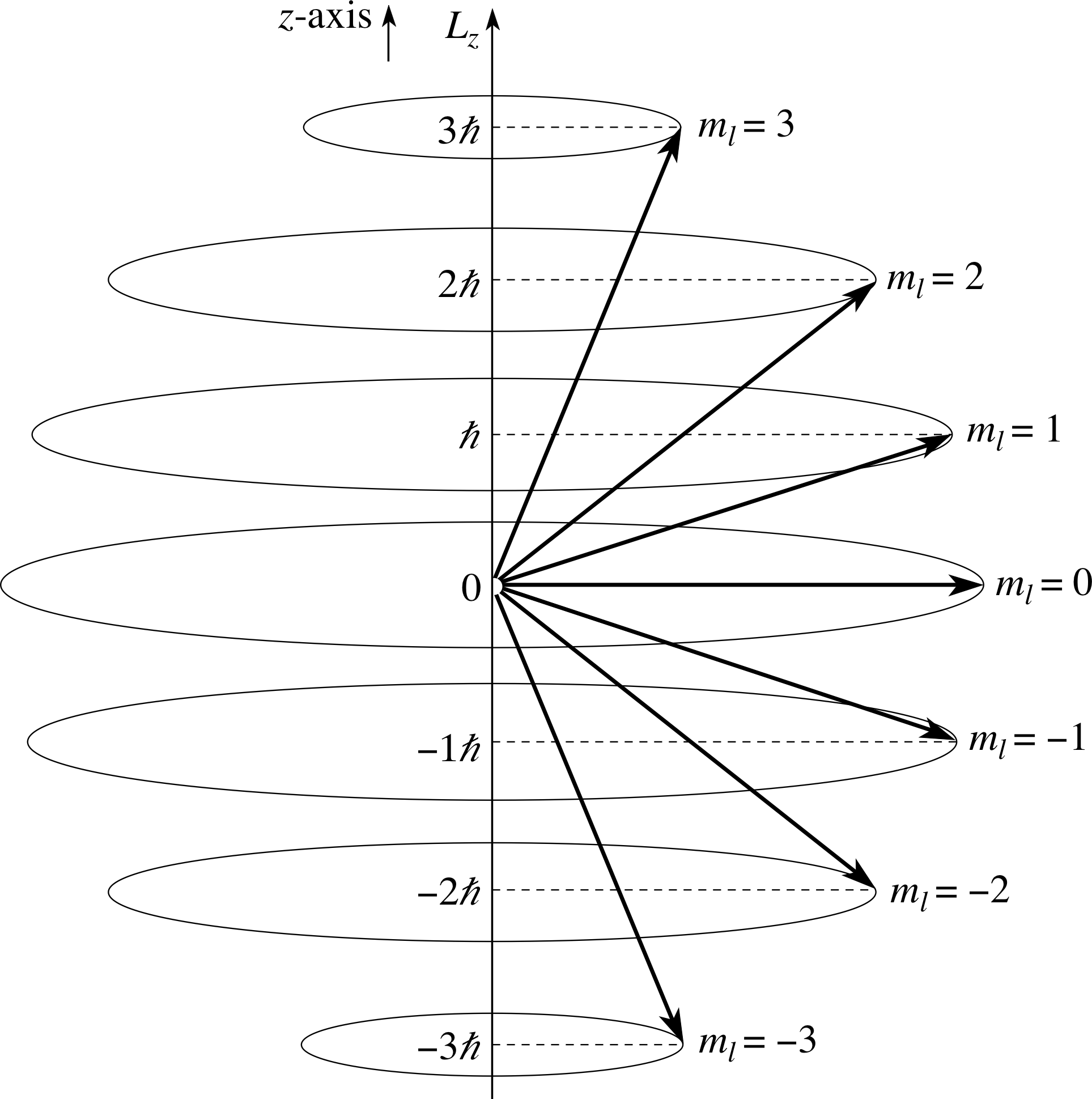
Figure 8 The orientations of angular momentum for l = 3 for the seven permitted values of Lz and ml.
Figure 7 The radial function Rnl(r) for the hydrogen atom for cases with principal quantum number n equal to 1, 2 and 3, and angular momentum quantum number l equal to zero. Note that the function Rn0(r) has n − 1 zeros (excluding the limit r → ∞).
3.3 Qualitative solutions of the Schrödinger equation – the electron distribution patterns
We will briefly illustrate some of the spatial properties of the electron in the hydrogen atom as predicted by the Schrödinger model. Remember that the spatial wavefunction of the state determined by the quantum numbers n, l, ml is given by ψnlm(r, θ, ϕ) = Rnl (r) Ylm(θ, ϕ). We have shown some examples of the radial functions, Rnl (r), in Figure 7. We also have to remember that in a stationary state the spatial wavefunction determines the probability of finding the electron in any region.
In three dimensions, | ψnlm(r, θ, ϕ) |2 is the probability per unit volume. The wavefunction can therefore be used to calculate the probability per unit volume of finding the electron in the region of each point specified by the coordinates (r, θ, ϕ). Since | ψnlm(r, θ, ϕ) |2 is equal to | Rnl (r) |2 × | Ylm (θ, ϕ) |2, we may consider the radial and angular parts separately.
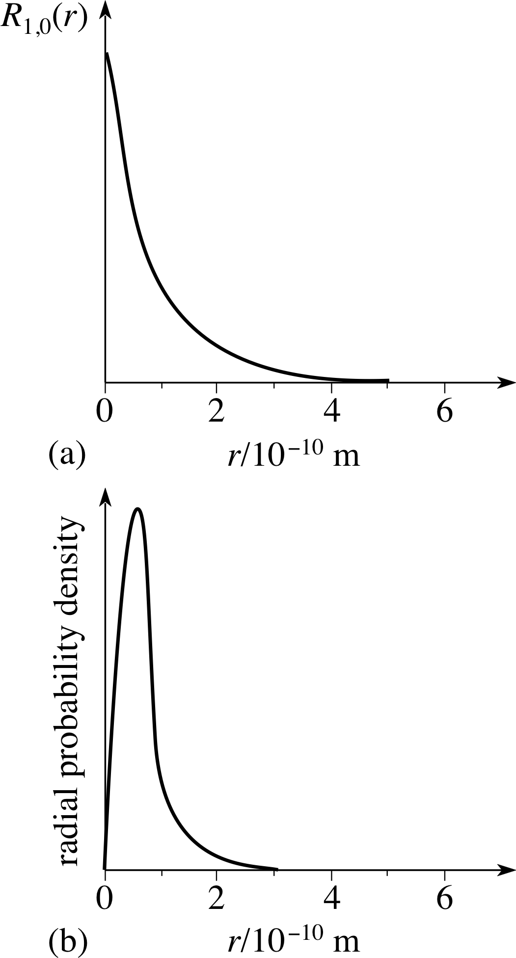
Figure 10 The radial wavefunction and the radial probability density for the n = 1, l = 1 electron in the hydrogen atom.
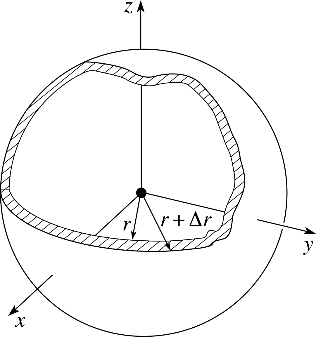
Figure 9 A sphere of radius r has surface area 4πr2. So, a thin spherical shell of radius r and thickness ∆r has volume 4πr2∆r.
The radial probability density
Consider first the case in which the probability density | ψnlm(r, θ, ϕ) |2 is independent of θ and ϕ; this will be true if l = 0. In such cases the function Rnl (r) will determine the probability Pnl (r) ∆r of finding the electron anywhere in the thin spherical shell of radius r and thickness ∆r, centred on the proton, as shown in Figure 9. Since | Rnl (r) |2 will be effectively constant over this shell we can write:
Pnl (r) ∆r = | Rnl (r) |2 4πr2 ∆r
In all cases, even when l ≠ 0, the function Pnl (r) = Pnl (r) ∆r = 4πr2 | Rnl (r) |2 is known as the radial probability density. We may therefore sketch the radial probability density, 4πr2 | Rnl (r) |2, if the radial wavefunction is known.
For example, Figure 10a repeats the radial wavefunction R1,0 (r) (n = 1, l = 0) and beneath it – Figure 10b – is sketched the corresponding radial probability density. The maximum of the radial wavefunction occurs at r = 0, but the maximum radial probability density occurs at r ≠ 0. This arises because the radial probability density is obtained by multiplying | Rnl (r) |2 by a function of r2, so the radial probability density is always set at zero at r = 0.

Figure 7c The radial function Rnl (r) for the hydrogen atom for cases with principal quantum number n equal to 3 and angular momentum quantum number l equal to zero.
Question T5
Figure 7c shows the radial wavefunction R3,0 (r) for the n = 3, l = 0 radial state. Sketch the radial probability density.
[Remember that the factor r2 in Pnl (r) ∆r = 4πr2 | Rnl (r) |2 ∆r means that the radial probability density at r = 0 is always zero.]

Figure 16a See Answer T5.
Answer T5
The radial probability density is shown in Figure 16a (see also Figure 7c). Note the increase in the size of the maxima of the radial probability density with r. This is because of the r2 term in
Pnl (r) ∆r = | Rnl (r) |2 4πr2 ∆r
The angular probability density
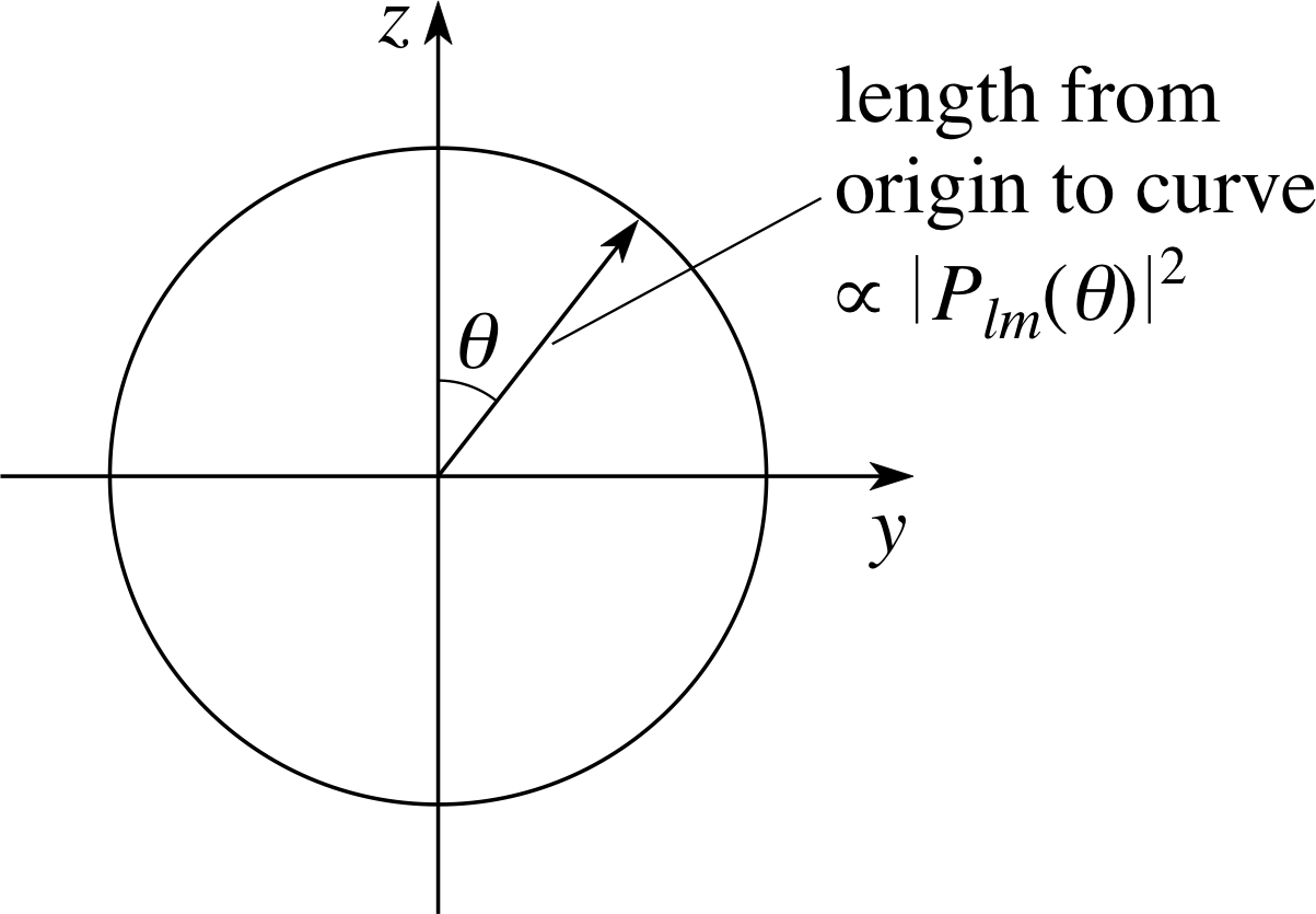
Figure 11 Polar diagram of the angular probability density for an l = 0 electron (an s electron).
The angular wavefunction, Ylm (θ, ϕ), consists of the product of two factors involving θ and ϕ separately:
Ylm(θ, ϕ) = Plm(θ) eimϕ
where Plm(θ) are polynomial functions, whose detailed form need not concern us here.
Because | eimϕ |2 = 1, the angular probability density:
| Ylm (θ, ϕ) |2 = | Plm(θ) |2
is independent of ϕ. i
For l = 0, | Plm (θ) |2 = | P0 0(θ) |2, which is independent of θ.
The angular dependence of the probability density may be represented by a polar diagram in which the lengths of vectors from the origin are made proportional to the value of | Plm(θ) |2 in the direction of the vectors. So, as shown in Figure 11, the polar diagram for l = 0 indicates, the vector has the same length in any direction, i.e. for any value of θ. The corresponding probability distribution | ψn 0 0 (r, θ, ϕ) |2 is therefore spherically symmetrical; it has the same dependence on r in every direction independent of θ and ϕ.
Before going on to other l–values, we will explain the notation that is usually used to indicate electron states. Rather than write out in full, say, n = 3, l = 2, each state is labelled with an integer, which is the n–value, and a letter, which gives the l value (see Table 3).
| orbital angular momentum quantum number, l | ||||||
| 0 | 1 | 2 | 3 | 4, 5, 6, ... | ||
| spectroscopic notation |
s | p | d | f | and thereafter alphabetical: |
g, h, i, ... |
| (sharp) | (principal) | (diffuse) | (fundamental) | |||
The electron in the state with n = 3, l = 2 will therefore be referred to as a 3d electron. The letters for the states l = 0 to l = 3 have a historical origin: sharp, principal, etc. refer to spectral lines resulting from electron transitions involving the designated states.
| orbital angular momentum quantum number, l | ||||||
| 0 | 1 | 2 | 3 | 4 | ||
| principal | 4 | 4d | ||||
| quantum | 3 | 3g | ||||
| number, | 2 | 2p | ||||
| n | 1 | 1s | ||||
Question T6
Correct and complete Table 4 with the appropriate spectroscopic notation for the electron with appropriate quantum numbers.
| orbital angular momentum quantum number, l | ||||||
| 0 | 1 | 2 | 3 | 4 | ||
| principal | 4 | 4s | 4p | 4d | 4f | |
| quantum | 3 | 3s | 3p | 3d | ||
| number, | 2 | 2s | 2p | |||
| n | 1 | 1s | ||||
Answer T6
The completed Table 4 is shown as Table 9:
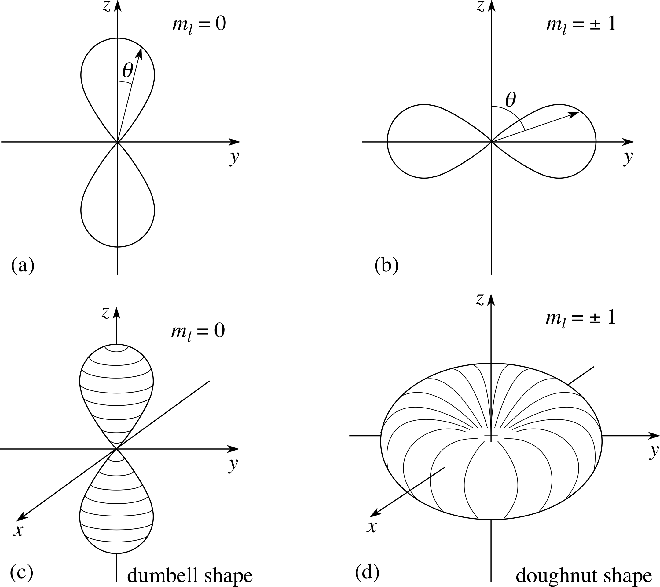
Figure 12 Polar diagrams of the angular probability density for a 2p electron, where | Plm(θ) |2 does vary with θ. (a) ml = 0, (b) ml = ±1, (c) ml = 0 rotated around z–axis, (d) ml = ±1 rotated around z–axis.
For l–values other than zero, Plm(θ) does depend on θ and also on ml. In particular, for l = 1, Figure 12a shows how this is represented by a polar diagram for l = 1, ml = 0. Figure 12a shows that the probability density has appreciable values only in the region of positive and negative z–directions (i.e. near θ = 0 and θ = π). For l = 1, ml = ±1, the probability density is only appreciable in the region near θ = π/2 as in Figure 12b. In both cases, the plot has been shown in the (y, z) (i.e. ϕ = 0) plane.
Since the probability density does not depend on ϕ at all, the full angular probability densities can be obtained by rotating these figures around the z–axis, as shown in Figures 12c and 12d.
An electron cloud picture for any state represents the product of the appropriate radial and angular probability densities as a cloud of varying density. For instance, Figure 13 shows a section through the electron cloud picture for the n = 2, l = 1, ml = ±1 state, and a section of the cloud for n = 3, l = 0 state is shown in Figure 16b (see answer to Question T5).
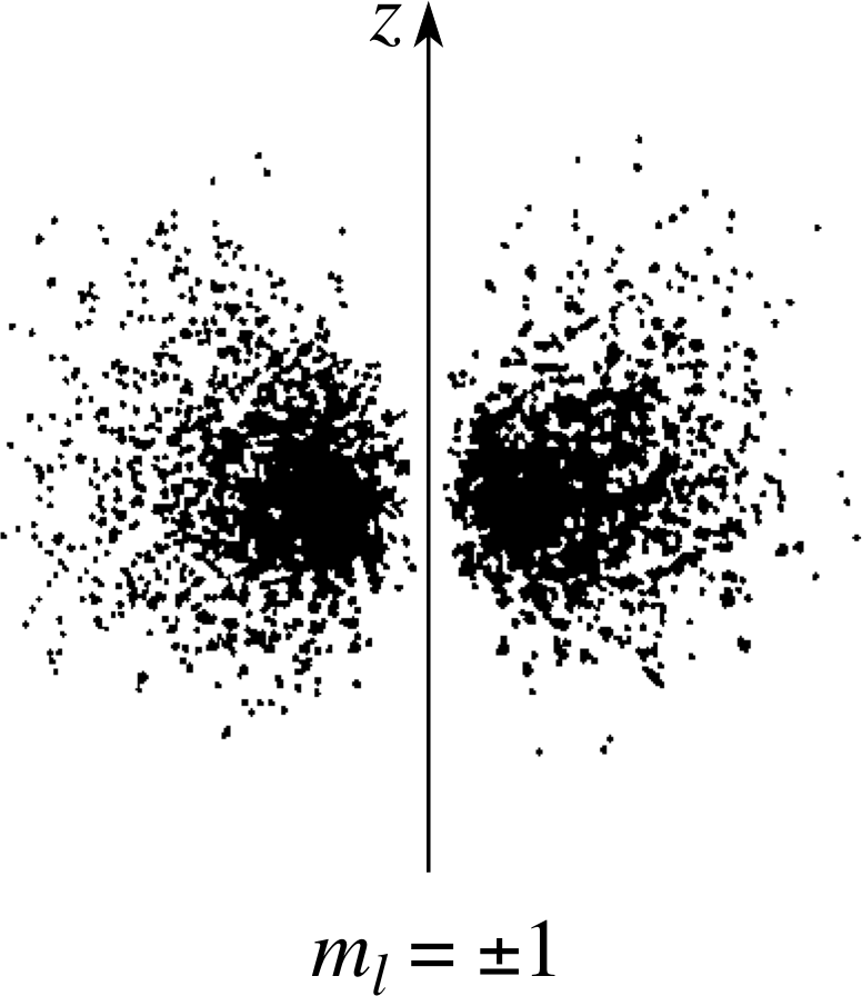
Figure 13 Electron cloud picture for the n = 2, l = 1, ml = ±1 states. (As usual only a section in the (x, y) plane is shown.)
Question T7
Using Figures 13 and 12c, sketch a section through the electron cloud picture for electrons in the n = 2, l = 1, ml = 0 state.
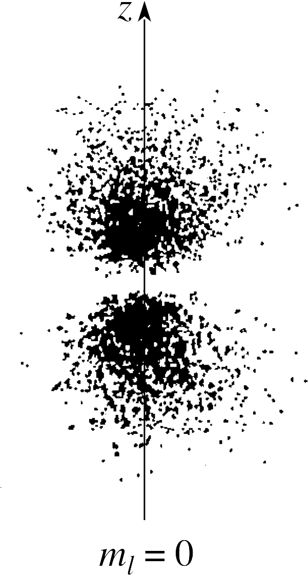
Figure 17 See Answer T7.
Answer T7
The electron cloud picture is shown in Figure 17.
3.4 Ionization and degeneracy
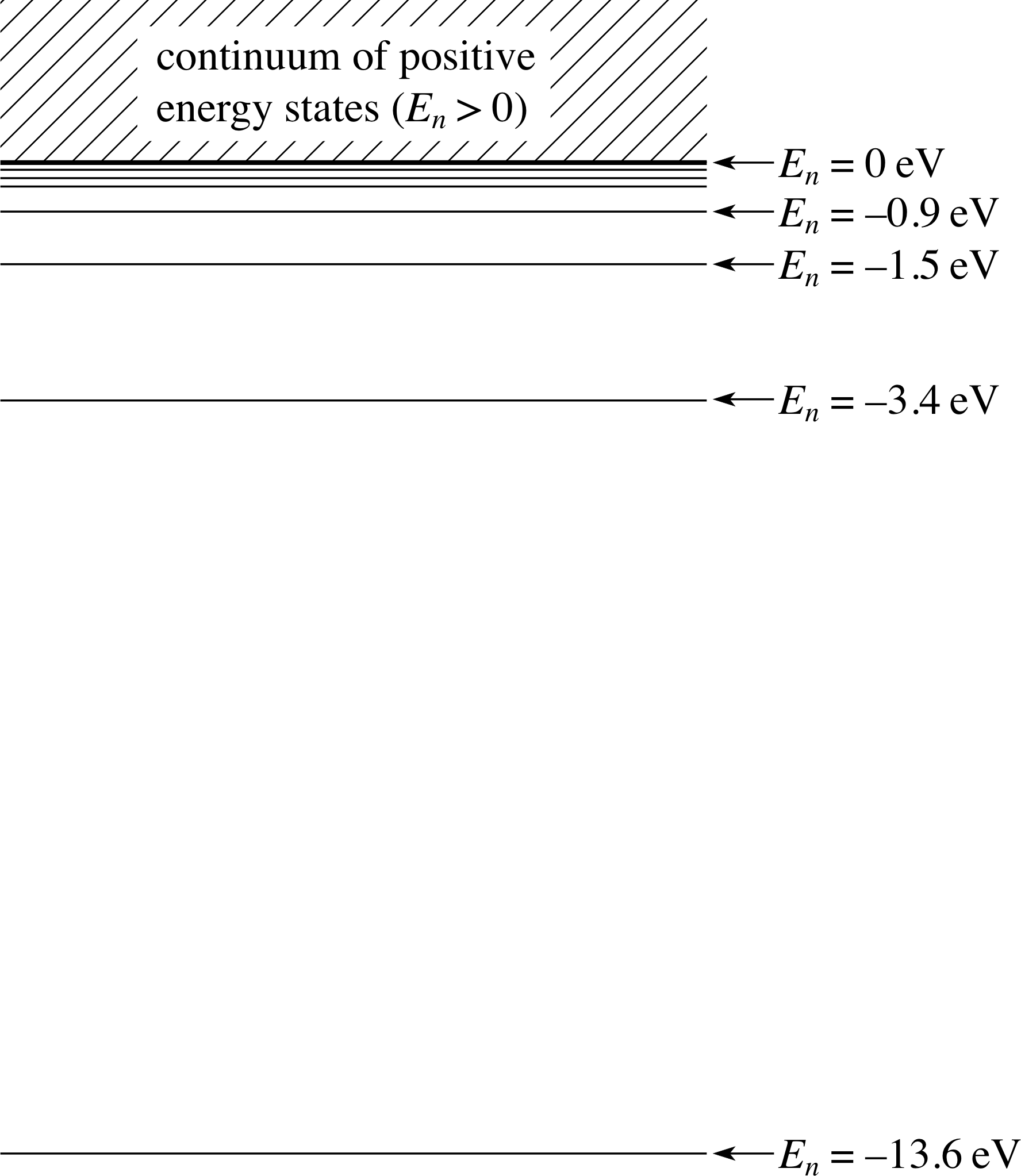
Figure 14 Energy levels of the electron in the hydrogen atom. The lowest energy level is n = 1 and consecutive levels are n = 2, n = 3, etc.
We saw in Subsections 2.1 and 3.2 that the energy values allowed for the electron in the hydrogen atom are given by:
$E_n = \dfrac{m_{\rm e}e^4}{8\varepsilon_0^2h^2}\dfrac{1}{n^2}$ n = 1, 2, 3, ...(Eqn 6)
or in units of electronvolts,
$E_n = -\dfrac{\rm 13.6\,eV}{n^2}$ n = 1, 2, 3, ...(Eqn 6a)
These are total energies for the bound states of the hydrogen atom and so must be negative.
The ground (lowest energy) state has energy −13.6 eV. The first excited state has energy −3.4 eV, and so on.
Question T8
How much energy must be given to an electron in the ground state to raise it to (a) the first excited state, (b) the second excited state?
Answer T8
The energy is given by En = −13.6 eV/n2. The ground (lowest) state has quantum number n = 1. Its energy is therefore E1 = −13.6 eV. The first and second excited states have energies of, respectively, E2 = −3.4 eV and E3 = −1.5 eV. The energies required are therefore,
(a) −3.4 eV − (−13.6 eV) = 10.2 eV, and
(b) −1.5 eV − (−13.6 eV) = 12.1 eV.
| Value of n |
Values of l |
Values of ml |
Number of states for each n and l |
Number of states for each n |
|---|---|---|---|---|
| 1 | 0 | 0 | 1 | 1 |
| 2 | 0 | 0 | 1 | 4 |
| 1 | −1, 0, 1 | 3 | ||
| 3 | 0 | 0 | 1 | 9 |
| 1 | −1, 0, 1 | 3 | ||
| 2 | −2, −1, 0, 1, 2 | 5 | ||
| 4 |
As more and more energy is given to the electron, its total energy becomes less and less negative. The electron also becomes less and less firmly attached to the proton. Eventually, it may be given just enough energy to escape from the influence of the proton – the hydrogen atom is then said to have just been ionized. The energy of the electron will then be zero – it will be free from the proton but will have no surplus kinetic energy. i The Schrödinger equation has solutions for total energies greater than or equal to zero. There are however no quantization restrictions on the positive energies of a free electron. Sometimes these unbound states of positive energy are described as continuum states since they correspond to a continuous range of energy levels, shown shaded on Figure 14. Figure 14 also shows the complete spectrum of bound state energy levels for the electron.
We know from Subsection 3.3 that there is usually more than one electron state corresponding to a given energy value. This is because the energy is determined only by the principal quantum number n, and, for a given n, there are several possible wavefunctions corresponding to different states (l, ml) of angular momentum. Table 5 shows how the number of states is made up for the smaller n values.
Question T9
Complete Table 5 for n = 4. Can you see a pattern building up relating the number of states for each value of n?
| Value of n |
Values of l |
Values of ml |
Number of states for each n and l |
Number of states for each n |
|---|---|---|---|---|
| 1 | 0 | 0 | 1 | 1 |
| 2 | 0 | 0 | 1 | 4 |
| 1 | −1, 0, 1 | 3 | ||
| 3 | 0 | 0 | 1 | 9 |
| 1 | −1, 0, 1 | 3 | ||
| 2 | −2, −1, 0, 1, 2 | 5 | ||
| 4 | 0 | 0 | 1 | 16 |
| 1 | −1, 0, 1 | 3 | ||
| 2 | −2, −1, 0, 1, 2 | 5 | ||
| 3 | −3, −2, −1, 0, 1, 2, 3 | 7 |
Answer T9
The solution is given in Table 10. If you look at the totals in the final column, you will see that there are n2 states corresponding to principal quantum number n.
[We have illustrated special cases of the arithmetic series summation: 1 + 3 + 5 + ... + (2n − 1) = n2, since it may be seen from the penultimate column of Table 10 that, for a given n, the number of states is the sum of the odd integers from one to 2n − 1.]
Wavefunctions which share a common energy level are said to be degenerate. In hydrogen, degeneracy exists for all (l, ml) combinations for each n value. The number of such combinations is said to be the order of degeneracy for the energy level. For atoms other than hydrogen the potential energy function is more complicated since each electron interacts with all other electrons as well as with the nucleus. The result is that the energies depend on l as well as n and are less degenerate.
The degeneracy of levels has experimentally detectable consequences. We noted in Subsection 3.2 that the choice of an axis, usually labelled the z–axis, is arbitrary. This is because of the spherical symmetry of the Schrödinger equation for the hydrogen atom. This is in turn reflected by the fact that for a given l, the energy has the same value for each value of ml. The directional (i.e. z–component) quantum number ml has no effect on the energy. The situation is changed, however, if the spherical symmetry is broken. One way to do this is to place the hydrogen atom in a uniform magnetic field. Now there is only symmetry of rotation about one axis – the direction of the field – rather than about any axis as before. Now there is a physically determined axis from which to make measurements of θ – a physical z–axis. Of course, we are now dealing with a changed case because the electron will interact with the magnetic field. The energy of the electron will be found to depend on ml as well as on l. Consequently, it is predicted that transitions involving an initial and final state of given l–values will now give rise to several different wavelengths depending on the initial and final ml values instead of a single wavelength. This splitting of the energy levels in a magnetic field leads to the splitting of the observed spectral lines and is known as the Zeeman effect. i The number of components into which each line is split is consistent with the 2l + 1 values of ml for each l. This follows naturally as part of the Schrödinger model.
3.5 Comparison of the Bohr and the Schrödinger models of the hydrogen atom
In Table 6, we summarize the comparison between the Bohr and the Schrödinger models. Test yourself by only revealing the entries in columns two and three (by clicking on each table cell) when you have thought of your own answers.
| Bohr’s model | Schrödinger’s model | |
|---|---|---|
|
1 What are the energy levels of the |
$E_n = -\dfrac{13.6}{n^2}\rm\,eV$ where n is Bohr’s quantum number; n = 1, 2, ... |
$E_n = -\dfrac{13.6}{n^2}\rm\,eV$ where n is the principal quantum |
|
2 What are the possible values of |
$n\hbar$ n = 1, 2, ... |
$\sqrt{l(l + 1)\os}\hbar$ l = 0, 1, 2, ... , n − 1 |
|
3 Can the electron have zero |
No, the minimum value is $\hbar$ |
Yes, for l = 0. |
|
4 What quantum numbers specify |
Bohr’s quantum number; n = 1, 2, ... |
n, l and ml n = 1, 2, ... l = 0, 1, 2, ... , n−1 ml = 0, ±1, ±2, ... , ±l |
|
5 What is the role of the electron’s |
It specifies the magnitude of the electron’s |
It specifies the electron’s energy |
|
6 What is the role of the quantum |
No role. |
It specifies the magnitude of the $L^2 = l(l+1)\hbar^2$ |
|
7 What is the role of the quantum |
No role. |
It specifies the z–component of the $L_z = m_l\hbar$ |
Question T10
How many states of the electron in the hydrogen atom are there with angular momentum of magnitude $3\hbar$ according to (a) the Bohr model, and (b) the Schrödinger model?
[Hint: Think carefully before you answer this question!]
Answer T10
(a) In the Bohr model, there is one state with orbital angular momentum of magnitude 3. It is the state with quantum number n = 3. Its energy is
E = −13.6 eV/32 = −1.5 eV
(b) In the Schrödinger model, the magnitude of the orbital angular momentum is $\sqrt{l(l+1)\os}$ with l an integer. The magnitude is therefore never equal to an integral multiple of . In particular, there are no states with orbital angular momentum equal to 3.
You will see that the apparent success of the Bohr model was only ‘skin deep’. The energy values did have the same form as those found in the Schrödinger model, but the quantum number n was incorrectly identified with the angular momentum. No zero angular momentum states were identified, and all states were labelled by a single quantum number. To be fair, the Bohr model was restricted in its scope. It was essentially a two–dimensional model: the electron was moving in a circular orbit in a plane. However, this is part of classical physics. A particle moving in a central field – such as the Coulomb field in this case – must be confined to a plane. The classical model can be extended to include elliptical orbits, but the orbit will still be confined to a plane. There is no possibility in classical physics that an orbit with zero orbital angular momentum can be produced.
In the Schrödinger case, l = 0 states are possible. They are the spherically symmetrical states. The electron is not confined to a plane; it has a probability of being found in any direction from the proton at the origin – a probability proportional to | Rn 0 (r) |2. It may be envisaged as having instantaneous angular momentum, which, because of the symmetry of the state, averages to zero.
The other feature of note in the Schrödinger model is the existence of several distinct states for each energy level. For the level labelled by the principal quantum number n, there are n2 states labelled by the allowed values of l and ml. In the language of quantum mechanics, the levels are said to be n2–fold degenerate. Degeneracy does not occur in the Bohr model.
The Schrödinger model has many other features that do not even see the light of day in the Bohr model, especially the Zeeman effect and the prediction of the intensities of the spectral lines. However that is beyond the scope of this module.
3.6 The classical limit
Figure 1 Four of the standing waves that may be set up on a taut, elastic string that is fixed at each end. The diagrams are not to scale, and are only snapshots of the waves, each of which varies with time.
We must now ask how this quantum model of the atom fits in with classical ideas. This is necessary because we could construct a quantum model of the motion of the Moon round the Earth, or of the Earth round the Sun, in just the same way as we have modelled the hydrogen atom; the fact that the gravitational potential energy varies with distance in exactly the same way as electrostatic potential energy makes this simple. In classical physics, we are dealing with much larger quantities than are relevant to individual atoms, so that we should look first of all at what happens to the theory in the regime of large quantum numbers.
Before we deal with atoms, let us recall what happens when we have a particle confined to a one–dimensional box. The spatial wavefunctions take the form of sine waves, as illustrated by Figure 1. As more and more energetic particles are considered, the spatial wavefunctions have more and more zeros and maxima, so that, provided we do not look at it in too great detail, the probability of finding the particle at any point in the box becomes constant, which is what we should expect classically. In this case, then, it looks as if it is possible to make a transition from quantum to classical mechanics without too much difficulty.
Now, returning to the atom, since the Bohr model gives numbers of the right order of magnitude for physical quantities, and simple formulae, let us use it to consider what happens in the limit of large values for n.
We have for the nth Bohr orbit:
$r = n^2\dfrac{\varepsilon_0h^2}{\pi m_{\rm e}e^2} \equiv n^2a_0$(Eqn 4)
$E_n = - \dfrac{\rm 13.6\,eV}{n^2}$(Eqn 6a)
and$L = m\upsilon_nr_n = n\hbar$(Eqn 1)
so that$\upsilon_n = \dfrac{\hbar}{ma_0n} = \dfrac{\upsilon_1}{n}$
We can now see how big the changes in these quantities are when the electron moves from Bohr orbit (n − 1) to orbit n.
$\Delta r = r_n - r_{n-1} = a_0(n^2 - (n - 1)^2) = (2n - 1)a_0$
$\Delta E = E_n - E_{n-1} = E_1\left(\dfrac{1}{n^2} - \dfrac{1}{(1-n)^2}\right) = \dfrac{-(2n-1)E_1}{n^2(n-1)^2}$
$\Delta\upsilon = \upsilon_n - \upsilon_{n-1} = \upsilon_1\left(\dfrac1n - \dfrac{1}{1-n}\right) = \dfrac{-\upsilon_1}{n(n-1)}$
When n is very large, we can neglect 1 compared to n, and these equations simplify to:
$\Delta r \approx 2na_0\quad\text{or}\quad\dfrac{\Delta r}{r} = \dfrac2n$ since r = n2a0
$\Delta E \approx \dfrac{-2E_1}{n^3}$
$\Delta\upsilon \approx \dfrac{-\upsilon_1}{n^2}$
✦ What do these quantities amount to if we take n = 106?
✧ Remembering that a0 = 0.53 × 10⁻¹⁰ m, E1 = −13.6 eV, and calculating that υ1 = 2.18 × 10⁶ m s−1, we find rn = 1012 × 0.53 × 10−10 m = 53 m (a very large hydrogen atom!)
υn = 2.18 m s−1 ∆r/r = 2 ×10⁻⁶, or ∆r ≈ 10−4 m ∆E ≈ 2.7 × 10⁻¹⁷ eV ∆υ ≈ −2 × 10⁻⁶ m s−1 so that when the change in orbital radius is just approaching visibility, the changes in energy and electron speed are negligibly small.
In fact, we can treat all these quantities as varying continuously for sufficiently large n. This situation would be indistinguishable from classical predictions.
Question T11
The gravitational potential energy of two bodies of masses m and M at a distance r apart is Epot = −GmM/r, where G, the gravitational constant and has the value G = 6.67 × 10⁻¹¹ N m2 kg−2. Consider a satellite of mass mS of 6.0 × 10³ kg in orbit around the Earth, 100 km above the equator. Repeat Bohr’s calculation using a gravitational rather than an electrostatic force. Take the mass of the Earth me to be 6.0 × 1024 kg, and its equatorial radius to be 6.4 × 10⁶ m.
(a) What is the value of n for the satellite orbit?
(b) If the satellite makes a transition from orbit n to orbit (n − 1), what is the change in the radius of the orbit?
(c) What is the corresponding change in the speed of the satellite?
Do not be alarmed by the size of the numbers that appear!
Answer T11
(a) The only change necessary in the calculation outlined in Subsection 2.1 is the replacement of the force term appearing in Equation 2, e2/(4πε0r2), by the gravitational equivalent GmM/r2.
Equating $\dfrac{m_{\rm S}\upsilon^2}{r} = \dfrac{Gm_{\rm S}m_{\rm E}}{r^2}\quad\text{with}\quad n^2\hbar^2 = m_{\rm S}^2\upsilon^2r^2 (=L^2) = m_{\rm S}r^3\dfrac{Gm_{\rm S}m_{\rm E}}{r^2}$
$n\hbar^2 = Gm_{\rm S}^2m_{\rm E}r$
so$n^2 = \dfrac{Gm_{\rm S}^2m_{\rm E}r}{\hbar^2}\\ \phantom{n^2 }= \rm \dfrac{6.67\times10^{-11}\,N\,m^2\,kg^{-2}\times(6.0\times10^3)^2\,kg^2\times6.0\times10^{24}\,kg\times(6.4+0.1)\times10^6\,m}{(6.63\times10^{-34}\,J\,s/2\pi)^2}\\ \phantom{n^2 }= 8.41\times10^{96}\,m$
so $n = 2.90\times10^{48}$
(b) The change in radius is ∆r = −2r/n = −4.5 × 10−42 m.
(c) $\upsilon = \hbar/nma_0 = \rm 7848\,m\,s^{-1}$, so that ∆υ = υ/n = 2.7 × 10−45 m s−1.
From these calculations, it should be clear that provided the quantum numbers are large enough, the discontinuities and other special feature of quantum mechanics become invisible, and a physical system will behave in the well–established classical manner. This fact is an example of the correspondence principle:
The correspondence principle
In the limit of large quantum numbers, (sometimes known as the classical limit), the predictions of quantum mechanics are in agreement with those of classical mechanics. i
4 Closing items
4.1 Module summary
- 1
-
The four postulates of the ‘semi-classical’ Bohr model lead to the quantization of the total energy of the electron in the hydrogen atom.
- 2
-
The postulate restricting the orbital angular momentum of an electron in the Bohr model may be related to the stationary configuration in which a whole number of de Broglie wavelengths of the electron fit into the circumference of the corresponding Bohr orbit.
- 3
-
The solutions of the time–independent Schrödinger equation in spherical polar coordinates for the electron in the hydrogen atom have two factors. The radial factor Rnl (r) depends only on r, and is determined by the principal quantum number n and the orbital angular momentum quantum number l. The angular part Ylm(θ, ϕ) depends on θ and ϕ and is determined by l and the magnetic quantum number ml.
- 4
-
The function Ylm(θ, ϕ) is the eigenfunction for angular momentum. The magnitude of the angular momentum squared has permitted values $L^2 = l(l + 1)\hbar^2$; its z–component is $L_z = m_l \hbar$ where ml can take on the 2l + 1 permitted values −l, −l + 1, ... , −1, 0, 1, ... , l − 1.
- 5
-
For each n, there are n permitted values of l: 0, 1, 2, ... , n − 1.
- 6
-
The energy of the electron depends only on n. It is quantized with levels En = −13.6 eV/n2 where n may be any positive integer: 1, 2, 3, ....
- 7
-
Radial probability density and angular probability density functions can be defined as Pnl (r) = | Rnl (r) |2 × 4πr2 and | Ylm(θ, ϕ) |2 respectively and these can be shown graphically and as electron cloud pictures.
- 8
-
There are several states corresponding to each energy, except for the case n = 1, since more than one set of values of l and ml correspond to each n. In fact there are n2 states corresponding to energy En. The level is n2–fold degenerate.
- 9
-
The Bohr and the Schrödinger models predict the same energy levels but differ in the number and angular momenta of the states corresponding to each level.
- 10
-
According to the correspondence principle, for sufficiently large quantum numbers the predictions of quantum theory and classical theory are the same.
4.2 Achievements
Having completed this module, you should be able to:
- A1
-
Define the terms that are emboldened and flagged in the margins of the module.
- A2
-
State the postulates of the Bohr model for the hydrogen atom; indicate which are purely classical and which are not.
- A3
-
Relate the orbital angular momentum postulate of the Bohr model to the stationary de Broglie waves of the electron in an orbit.
- A4
-
Write down the time–independent Schrödinger equation for the electron in the hydrogen atom (Equation 17).
- A5
-
Identify the quantum numbers n, l and ml that label the spatial wavefunction solutions of the time–independent Schrödinger equation for the hydrogen atom.
- A6
-
State the physical variables to which each of the quantum numbers relates and the values these quantities are permitted to have.
- A7
-
State the permitted values of the quantum numbers and determine the number of states corresponding to any given value of n.
- A8
-
Figure 8 The orientations of angular momentum for l = 3 for the seven permitted values of Lz and ml.
Draw diagrams showing the relationship between the orbital angular momentum vector and its z–component (see Figure 8).
- A9
-
For sufficiently simple cases; sketch graphs of radial wavefunctions Rnl (r), and the corresponding radial probability densities, also draw polar diagrams of angular probability densities and sketch electron cloud pictures.
- A10
-
Write down the spectroscopic notation for any given electron state.
- A11
-
Compare and contrast the predictions of the Bohr model and the Schrödinger model.
- A12
-
State the formula for the energy levels, En, in terms of electronvolts (Eqn 6a),
En = −13.6 eV/n2 n = 1, 2, 3, ...(Eqn 6a)
- A13
-
Calculate the frequency or wavelength of the quanta of electromagnetic radiation emitted following an electron transition between two given energy states.
- A14
-
State and explain a simple version of the correspondence principle.
Study comment You may now wish to take the following Exit test for this module which tests these Achievements. If you prefer to study the module further before taking this test then return to the topModule contents to review some of the topics.
4.3 Exit test
Study comment Having completed this module, you should be able to answer the following questions each of which tests one or more of the Achievements.
Question E1 (A2 and A3)
State the four postulates of the Bohr model of the hydrogen atom. Indicate which are classical and which are quantum-mechanical. How may the orbital angular momentum of the electron be related to its de Broglie wavelength?
Answer E1
The five postulates are:
Postulate 1 The electron in the atom moves in a circular orbit centred on its nucleus which is a proton. Its motion in the orbit is governed by the Coulomb electric force between the negatively charged electron and the positively charged proton.
Postulate 2 The equation of motion of the electron is Newton’s second law of motion but the angular momentum of the electron in its circular orbit can only take values that are integer multiples of h/2π, where h is Planck’s constant. We may write: L = nh/2π.
Postulate 3 An electron in a Bohr orbit does not radiate electromagnetic radiation. Its energy is therefore constant. The orbit is referred to as a stationary orbit.
Postulate 4 Electromagnetic radiation is only emitted when the electron changes from one orbit to another of a lower total energy. (The electron is said to undergo a transition.) In such a case, the energy lost, ∆E, is emitted as one quantum of radiation of frequency f given by the Planck–Einstein formula: ∆E = hf.
Postulate 1 depends entirely on classical physics. Postulate 2 introduces a restriction on the orbital angular momentum in terms of Planck’s constant h. It is therefore quantum–mechanical in nature. Postulate 3 announces the suspension of classical laws for stationary orbits, while Postulate 4 states that the Planck–Einstein quantum formula applies for the radiation emitted in the course of a transition.
The stationary orbit may be thought of as one that contains a whole number n of de Broglie wavelengths of the ‘orbiting’ electron. If the consequences of this are worked out, the stationary orbit is found to have $n\hbar$ units of orbital angular momentum, corresponding to the second postulate of the Bohr model.
(Reread Subsections 2.1 and 2.2 if you had difficulty with this question.)
Question E2 (A4, A5 and A6)
Write down the Schrödinger equation for the electron in the hydrogen atom. Given that the solution can be written in the form Rnl (r) Ylm(θ, ϕ), name the quantum numbers and state how they relate to the physical quantities of the electron states.
Answer E2
The Schrödinger equation for the electron in the hydrogen atom is:
$-\dfrac{\hbar^2}{2m\os}\left(\dfrac{\partial^2}{\partial x^2}+\dfrac{\partial^2}{\partial y^2}+\dfrac{\partial^2}{\partial z^2}\right)\psi_{n\,l\,m}(x,\,y,\,z) - \dfrac{e^2}{4\pi\varepsilon_0r}\psi_{n\,l\,m}(x,\,y,\,z) = E\psi_{n\,l\,m}(x,\,y,\,z)$
The three quantum numbers that label different electron states are n, the principal quantum number, l, the orbital angular momentum quantum number, and ml, the magnetic quantum number.
The value of n determines the energy of the electron: En = −13.6 eV/n2.
The value of l determines the orbital angular momentum of the electron: $\sqrt{l(l+1)\os}\hbar$. The value of ml determines the value of the z–component of angular momentum: $m_l\hbar$
(Reread Subsections 3.1 and 3.2 if you had difficulty with this question.)
| Value of n | Values of l | Values of ml | Number of states for each n and l |
Number of states for each n |
|---|---|---|---|---|
| 3 |
Question E3 (A7)
What values of the quantum number n are permitted? Fill in Table 7 with the permitted quantum numbers for the state with n = 3. Complete the Table to show how many states correspond to this quantum number.
| Value of n | Values of l | Values of ml | Number of states for each n and l |
Number of states for each n |
|---|---|---|---|---|
| 3 | 0 | 0 | 1 | 9 |
| 1 | −1, 0, 1 | 3 | ||
| 2 | −2, −1, 0, 1, 2 | 5 |
Answer E3
The principal quantum number n may have any positive integer value: 1, 2, 3, 4, ... . The permitted values of l for a given n are: 0, 1, 2, ..., n − 1. For each value of l, ml may have the values: −l, −l + 1, ..., −1, 0, 1, ..., l − 1, l.
The completed Table 7 is therefore as shown: The Table shows that there are 9 states with n = 3. (This is a special case of the general result: the principal quantum number n is carried by n2 states.)
(Reread Subsections 3.1 and 3.2 if you had difficulty with this question.)
Question E4 (A8)
Draw a diagram showing the possible orientations of the orbital angular momentum vector corresponding to l = 1. Calculate the angles between the vectors and the z–axis, and show them on your diagram.
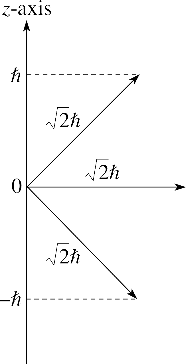
Figure 18 See Answer E4.
Answer E4
The value of the magnitude of the orbital angular momentum is $\sqrt{l(l+1)\os}\hbar$ so, for l = 1, this is $\sqrt{2\os}\hbar$.
The z–component is ml, in this case $-\hbar,~0,~\hbar$.
The orientations are shown in Figure 18. The angles are as shown. The angle between the vector with zero z–component and the z–axis is of course 90°. The other angles with the z–axis are equal to $\arccos(1/\sqrt{2\os}) = 45°$.
(Reread Subsection 3.2 if you had difficulty with this question.)
Question E5 (A9)
Sketch the graph of R2,0(r) as a function of r. Draw beneath it the radial probability density distribution corresponding to the wavefunction and the electron cloud picture for it.

Figure 7b The radial function Rnl (r) for the hydrogen atom for case with principal quantum number n equal to 2 and angular momentum quantum number l equal to zero. Note that the function Rn 0(r) has n − 1 zeros (excluding the limit r → ∞).
Answer E5
The radial wave function for the 2s electron is shown in Figure 7b. The radial probability density function and the electron cloud picture for the 2s electron are shown in Figures 19a and 19b, respectively.
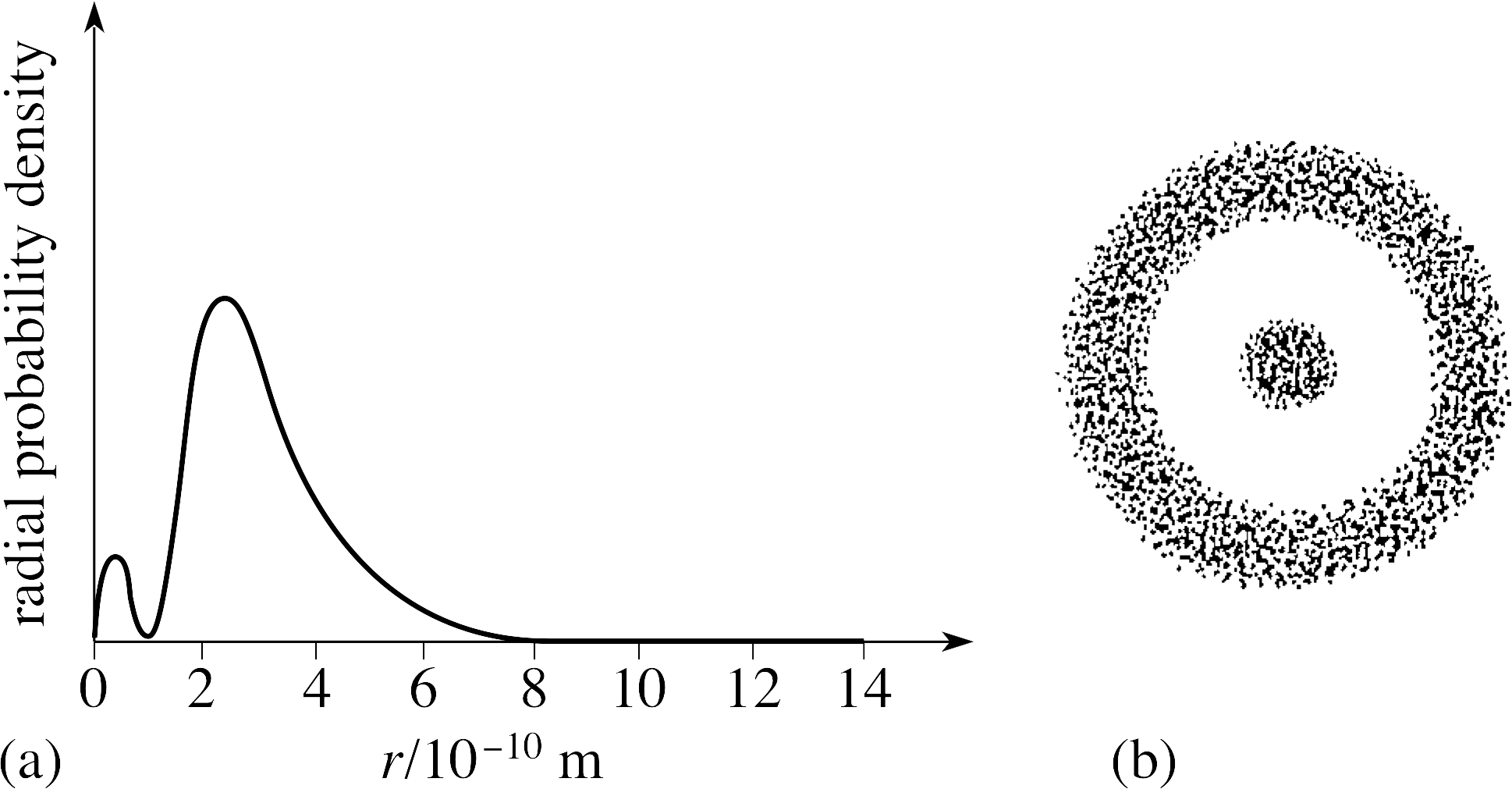
Figure 19 See Answer E5.
(Reread Subsection 3.1 if you had difficulty with this question.)
Question E6 (A10)
Write down the spectroscopic notation for the states involved in your answer to Question E3.
Answer E6
The quantum numbers of the relevant states were n = 3 with l = 0, 1 and 2.
The spectroscopic notation for these three states is: 3s, 3p and 3d, respectively.
(Reread Subsection 3.2 if you have difficulty with this question.)
Question E7 (A11) TO BE SORTED OUT!
Complete Table 8, which is a partially blanked out version of Table 6.
| Bohr’s model | Schrödinger’s model | |
|---|---|---|
|
1 What are the energy levels of the |
$E_n = -\dfrac{13.6}{n^2}\rm\,eV$ where n is Bohr’s quantum number; n = 1, 2, ... |
$E_n = -\dfrac{13.6}{n^2}\rm\,eV$ where n is the principal quantum |
|
2 What are the possible values of |
$n\hbar$ n = 1, 2, ... |
$\sqrt{l(l + 1)\os}\hbar$ l = 0, 1, 2, ... , n − 1 |
|
3 Can the electron have zero |
No, the minimum value is $\hbar$ |
Yes, for l = 0. |
|
4 What quantum numbers specify |
Bohr’s quantum number; n = 1, 2, ... |
n, l and ml n = 1, 2, ... l = 0, 1, 2, ... , n−1 ml = 0, ±1, ±2, ... , ±l |
|
5 What is the role of the electron’s |
It specifies the magnitude of the electron’s |
It specifies the electron’s energy |
|
6 What is the role of the quantum |
No role. |
It specifies the magnitude of the $L^2 = l(l+1)\hbar^2$ |
|
7 What is the role of the quantum |
No role. |
It specifies the z–component of the $L_z = m_l\hbar$ |
Answer E7
See Table 6.
| Bohr’s model | Schrödinger’s model | |
|---|---|---|
|
1 What are the energy levels of the |
$E_n = -\dfrac{13.6}{n^2}\rm\,eV$ where n is Bohr’s quantum number; n = 1, 2, ... |
$E_n = -\dfrac{13.6}{n^2}\rm\,eV$ where n is the principal quantum |
|
2 What are the possible values of |
$n\hbar$ n = 1, 2, ... |
$\sqrt{l(l + 1)\os}\hbar$ l = 0, 1, 2, ... , n − 1 |
|
3 Can the electron have zero |
No, the minimum value is $\hbar$ |
Yes, for l = 0. |
|
4 What quantum numbers specify |
Bohr’s quantum number; n = 1, 2, ... |
n, l and ml n = 1, 2, ... l = 0, 1, 2, ... , n−1 ml = 0, ±1, ±2, ... , ±l |
|
5 What is the role of the electron’s |
It specifies the magnitude of the electron’s |
It specifies the electron’s energy |
|
6 What is the role of the quantum |
No role. |
It specifies the magnitude of the $L^2 = l(l+1)\hbar^2$ |
|
7 What is the role of the quantum |
No role. |
It specifies the z–component of the $L_z = m_l\hbar$ |
(Reread Subsection 3.5 if you had difficulty with this question.)
Question E8 (A12 and A13)
Three energy levels of the hydrogen atom have values −13.6 eV, −0.544 eV and −0.136 eV. To what quantum numbers do they correspond? What are the wavelengths of the spectral lines that may result from all possible transitions between them? [h = 4.14 × 10⁻¹⁵ eV s, c = 3.00 × 10⁸ m s−1]
Answer E8
The levels correspond respectively to n = 1, n = 5 and n = 10 in the general energy level formula En = −13.6 eV/n2.
There are three possible transitions (i) n = 5 to n = 1, (ii) n = 10 to n = 1, (iii) n = 10 to n = 5.
The energy emitted in a transition is emitted as a quantum of radiation of frequency f given by: f = ∆E/h.
Since c = f λ, the corresponding wavelength is:
$\lambda = \dfrac cf = \dfrac{hc}{\Delta E}$
The values in the three cases are therefore:
(i) λ = 95.13 nm; (ii) λ = 92.25 nm; (iii) λ = 3.04 μm
(Reread Subsection 3.4 if you had difficulty with this question.)
Study comment This is the final Exit test question. When you have completed the Exit test go back and try the Subsection 1.2Fast track questions if you have not already done so.
If you have completed both the Fast track questions and the Exit test, then you have finished the module and may leave it here.
Study comment Having seen the Fast track questions you may feel that it would be wiser to follow the normal route through the module and to proceed directly to the following Ready to study? Subsection.
Alternatively, you may still be sufficiently comfortable with the material covered by the module to proceed directly to the Section 4Closing items.