PHYS 1.1: Introducing measurement |
PPLATO @ | |||||
PPLATO / FLAP (Flexible Learning Approach To Physics) |
||||||
|
1 Opening items
1.1 Module introduction
Although some areas of science consist mainly of description, most sciences, and especially physics, can’t stop at this level. Sooner or later, two or more descriptive explanations of a phenomenon will come into conflict. If science is to be more than a ‘my-explanation-is-as-good-as-yours’ argument, there has to be some way of choosing between those rival explanations. This is one place where measurement is crucial. At a more routine level, measurement is also essential to the everyday activity of both science and technology – without measurement, progress is almost impossible.
This module is concerned with the measurement of physical quantities. Section 2 describes the system of measurement units that is currently in use (usually referred to as SI units) and explains how some of the basic units of that system are defined and maintained in terms of internationally accepted standards. In Section 3 a distinction is made between the units and dimensions of a quantity, and the technique of dimensional analysis is introduced as a method of checking the plausibility of proposed relationships between physical quantities.
Whenever a measurement is made, an estimate of the uncertainty or error in the measurement should also be given (this is discussed in Section 4). Such estimates are of great importance when comparing a measurement (or a result obtained from a measurement) with a theoretical prediction, or when comparing results obtained in different experiments to see if they are consistent. This module describes the two types of experimental error – random and systematic – and explains how they can be estimated in various situations. It also discusses the use of significant figures in the writing of results so that any ambiguity in the accuracy or precision is removed or, at least, reduced. Finally, Section 5 covers errors in the counting of randomly occurring events, such as radioactive decays.
Study comment Having read the introduction you may feel that you are already familiar with the material covered by this module and that you do not need to study it. If so, try the following Fast track questions. If not, proceed directly to the Subsection 1.3Ready to study? Subsection.
1.2 Fast track questions
Study comment Can you answer the following Fast track questions? If you answer the questions successfully you need only glance through the module before looking at the Subsection 6.1Module summary and the Subsection 6.2Achievements. If you are sure that you can meet each of these achievements, try the Subsection 6.3Exit test. If you have difficulty with only one or two of the questions you should follow the guidance given in the answers and read the relevant parts of the module. However, if you have difficulty with more than two of the Exit questions you are strongly advised to study the whole module.
Question F1
In five identical experiments to find g, the magnitude of the acceleration due to gravity, the following results were obtained: 10.4 m s−2, 10.5 m s−2, 10.3 m s−2, 10.4 m s−2 and 10.6 m s−2. Estimate the random and systematic errors associated with this experiment. You may assume that the correct value of g (to two significant figures) is 9.8 m s−2.
Answer F1
The mean value of g is 10.4 m s−1 (to three significant figures); if the correct value of g is 9.8 m s−2, the systematic error is +0.6 m s−2. The spread of readings about the mean is roughly ±0.1 m s−2, so the random error is approximately ±0.1 m s−2.
Question F2
The mean number of births occurring each day in a certain hospital is 49. Assuming that births are equally likely at any time, estimate the typical range through which the actual numbers of births each day varies.
Answer F2
The square root of the mean number of births is 7. On about 68% of days, the number of births will lie within ±7 of the mean, if they are truly random events. So on just under 70% of the days, there would be between 42 and 56 births.
Question F3
The five quantities a, b, c, d and e are related by an equation of the form
$a = \dfrac{b-c^2}{d}+e$
If a is measured in N m s−1 and b in J s, what are the units and dimensions of c, d and e?
Answer F3
From the units of a and b, it follows that the dimensions of those two quantities are given by
[a] = M L2 T−3 and [b] = M L2 T−1
Thus, dimensional consistency requires
[c2] = [b] = M L2 T−1 so [c] = M1/2 L T−1/2
and suitable units for c would be kg1/2 m s−1/2 or (J s)1/2.
Similarly, [e] = [a] = M L2 T−3 and suitable units would be kg m2 s−3 or N m s−1.
Finally, [d ] = [b/a] = T2 and suitable units would be s2.
1.3 Ready to study?
Study comment Relatively little background knowledge is required to study this module, though it is assumed that you have a general understanding of the terms: acceleration, atom, energy, gravity, mass, pressure, radioactive, speed and temperature. In addition it is assumed that you have previously performed a wide range of simple calculations and that you know the meaning of the following mathematical terms: cancelling, decimal_numberdecimal, equation, factor, percentage, power_mathematicalpower, scientific notation (i.e. powers–of–ten notation) and square root. If you are uncertain about any of these terms you should review them now by reference to the Glossary, which will indicate where in FLAP they are developed. You should also be able to work in decimal_numberdecimal and scientific notation (powers-of-ten), to simplify and evaluate expressions involving power_mathematicalpowers, and to use a calculator to perform simple calculations, including finding percentages. The following questions will allow you to establish whether you need to review some of the topics before embarking on this module.
Question R1
Evaluate [(8 × 10−2) × (3 × 104)]/(4 × 102).
Answer R1
6 × 100 = 6.
Question R2
What is 42% of 0.15?
Answer R2
0.15 × (42/100) = 0.063. Percentages are simply fractions expressed in hundredths.
Question R3
Express 2 803 000 in scientific notation.
Answer R3
2.803 × 10⁶. (As you will see in the discussion of significant figures, it might be appropriate to include more zeros to the right of the last digit of this number.)
Question R4
Use your calculator to evaluate (3.487 × 10¹²)/(2.900 × 103) and express your answer using scientific notation.
Answer R4
1.202 × 10⁹ in scientific notation.
Question R5
Evaluate (15.2 + 18.8) × 10−5. Give your answer both in scientific notation and in decimal notation.
Answer R5
Scientific notation: 3.40 × 10⁻⁴.
Decimal notation: 0.000 340.
Question R6
If a population of fruit flies increases from 92 to 138 in a certain period, what percentage increase does this represent?
Answer R6
Increase = 138 − 92 = 46.
Percentage increase = (46/92) × 100% = 50%.
Question R7
Evaluate (0.2)2(0.5)3/(0.1)2.
Answer R7
(0.2)2(0.5)3/(0.1)2 = (0.2/0.1)2 × 0.5 × 0.5 × 0.5 = 4 × 0.125 = 0.5.
Comment If you had difficulty with any of these Ready to study questions, consult to the Glossary for further information and references about the terms used.
2 Units and standards
2.1 The importance of standards
Physics is the fundamental science that attempts to discover the basic laws that describe the behaviour of all forms of matter and energy in the Universe. It is concerned with developing models, i.e. ways of representing and predicting that behaviour. These models are largely quantitative, in other words, they involve measurement – not just qualitative description. However, people have long realized that there are many reasons why they should be able to measure things. How else, for instance, could they know the quantity of grain they had for sale, or the distance they would have to carry it to market, or the time it would take to walk there? The need to measure things existed long before the need to decide between contending theories in physics.
One consequence is that we have inherited numerous units of measurement (metre, yard, foot, inch, etc.) with definitions based on a variety of standards. Naturally, these standards have evolved over the centuries, from largely crude and variable measures to the highly precise international standards used in modern science. We no longer measure distances in terms of a man’s stride: we now have length standards that are accurate to 1 inch in 10 000 miles. The immensely impressive ‘stone calendar’ at Stonehenge has been superseded by an atomic clock which operates with an accuracy of 1 second in 30 000 years. This evolution of measurement standards has been absolutely essential for the development of science. Without a system of well–defined units based on precise, reproducible standards, scientists would find it impossible to communicate their findings to one another unambiguously. It is therefore essential that you become acquainted with the international system of units and standards in present–day use.
2.2 International system of units
Measurement can usually be reduced to a comparison of something of interest with some agreed standard. For instance, if you were to take the width of this sheet of paper as a unit of length, the lengths of all other objects could be related to this width. One object may be twice as long as the width of this paper (i.e. 2 ‘paper-widths’); a second may be three-and-a-half times as long (3.5 paper-widths); another may be a quarter as long (0.25 paper-widths). Once the unit is established, measurement becomes simply a matter of counting. So if I tell you that I am 8.4 paper–widths tall, you will have some idea of how tall I am, even though you haven’t seen me. But note that it is important for you to know what the unit of measurement is; furthermore, you need to have access to a ‘copy’ of it. Someone who did not know what the unit of measurement was, or who did not have access to the ‘standard’ paper-width, would have no idea what is meant by a height of 8.4 units. We need standards, and these standards must be known by everyone with whom we wish to communicate. But what standards should we choose?
Length
Early standards of length tended to be related to the size of the human body. For example, the width of the thumb became the ‘inch’, the length of a foot became a ‘foot’, and when measuring cloth it was convenient to define the distance from the nose to the end of the middle finger when the arm was outstretched as a ‘yard’. Such ‘personal’ standards, though conveniently portable, can obviously vary considerably from person to person. The next step was to have a yardstick, copies of which could be sent all over the country, with the result that a yard of cloth in Edinburgh would be more or less the same length as a yard of cloth in London. But what do we mean by ‘more or less’? To within 1/10 inch? Nobody is likely to grumble about that sort of uncertainty if they are buying cloth; but in science we may well want to measure smaller subdivisions. So the precision of our standard must be improved. The ultimate limit to the accuracy with which we can make a measurement (no matter how good the equipment) will always be determined by the uncertainty in the standard. i It is no good making a measurement to an accuracy of 1/100 inch, if the agreement as to what constitutes a standard yard is only good to 1/10 inch. Hence, as scientists have sought to make more and more accurate measurements, so they have also had to devise more and more precise measurement standards.
Nowadays, there is also a further requirement: our measurement standards should be international. Clearly, this was unimportant when different communities did not interact with one another. Today, however, if scientists in Europe are to understand the measurements of scientists in the USA or Japan, they must be acquainted with one another’s standards of measurement. Better still, they should all use the same standards. In 1960 it was formally agreed to standardize according to:
The Système International d’Unités. This system, usually abbreviated as SI units, is now in universal use by the scientific community. SI units are metric, i.e. based upon the metre as the unit of length. The kilogram and second are also SI units.
The history of the metric system dates back to Napoleonic France, where the metre was originally defined as one ten–millionth of the distance from the Equator to the North Pole along a meridian passing through Dunkirk and Barcelona, and hence also passing very close to Paris. This standard could not be lost, but it could hardly be called practical. So in 1889 it was officially decided to define the metre as the distance between two parallel marks inscribed on a particular bar made of the metal alloy platinum–iridium (chosen because of its exceptional hardness and resistance to corrosion). To ensure the reproducibility of measurements of this length, the bar had to be kept under specific conditions. For instance, it had to be supported so as to minimize deformations, and kept at a constant temperature (that of melting ice) so as to prevent expansion or contraction. This standard metre still exists. It is housed in the International Bureau of Weights and Measures at Sevres, near Paris. Copies of this bar, i.e. secondary standards, are in national standards offices throughout the world.
Even this, however, was not completely satisfactory. For although the length of an object could be compared with the standard metre to a precision of about two parts in ten million (by using a high–powered microscope to view the finely inscribed marks on the metre bar), this precision was still inadequate for some scientific purposes. In addition, making comparisons with a bar that had to be kept under specific conditions in a standards laboratory was still inconvenient. What was required was a standard that anyone (or at least, any scientist) could have access to in any laboratory, a standard that did not require copies to be made (hence eliminating the problem of inexact copies), and a standard that could be relied upon never to change.
In 1961, by international agreement, a new standard of length was defined, based on the characteristic wavelength of the orange–red light emitted by krypton atoms. The length of the standard metre bar was carefully measured in terms of the ‘wavelength of krypton light’ and it was agreed that exactly 1 650 763.73 wavelengths would constitute one metre. This number was chosen so that the old definition of the metre (as the distance between the two inscribed marks on the platinum–iridium bar), and the new definition of the metre (as a particular number of wavelengths of krypton light) were kept in agreement. The new definition provided a standard of length far more precise than the metre bar, and the krypton standard was readily available to laboratories all over the world, since krypton is present in the Earth’s atmosphere. The krypton wavelength can be called a natural unit since it depends on a particular natural property – namely, the fact that all atoms of a given kind are identical, and consequently always emit light of exactly the same colour.
However, during the 1970s it became clear that measurements of length made with the latest technology were limited not by the measuring techniques themselves, but rather by the definition of the metre in terms of the krypton wavelength. In other words, the new measuring techniques were potentially more precise than the standard of length. So in 1983 it was agreed to adopt yet another definition of the metre. This one was different from all those that had gone before, because instead of being based on a measurement, the new standard was tied to a defined value. The property chosen this time was the speed of light in a vacuum. Physicists are now convinced that the speed of light in a vacuum is a fundamental universal constant – i.e. its value is always the same, everywhere – and therefore perfect for use as a basic standard of measurement.
So nowadays, the speed of light in a vacuum is a defined quantity: in one second light travels exactly 299 792 458 metres. i Consequently the metre can be defined as the distance that light travels in a vacuum in 1/299 792 458 seconds. This definition is completely consistent with the previous, krypton–wavelength standard.
Time
Time is a more difficult quantity to measure than length. An interval of time can be used only once, and then it’s gone – unless, that is, we can find some periodic process, i.e. one that repeats with a regular and countable pattern. One possibility is to choose the mean solar day as the standard. The mean solar day is the average (taken over a year) of the time the Earth takes to spin once on its axis, relative to the Sun. The division of this mean solar day into 24 hours, and each hour into 60 minutes, and each minute into 60 seconds, then gives us the basic unit of time: the second. It is the second that has been adopted as the SI unit of time. This way of defining a unit of time in terms of the solar day has been adequate for the majority of everyday applications, but it has proved unsatisfactory for very high precision work. For, in addition to the variation in the solar day caused by variations in the Earth’s orbital speed, there is also a cumulative slowing down of the Earth’s spin (probably caused by tidal friction), the net effect of which is to cause our solar clock to lose over half an hour every 1000 years.
So in 1967, a natural unit of time was adopted. Like the natural unit of length, this natural unit of time was based upon the identical nature of all the atoms of a particular species – in this case, the atoms of caesium. Every atom vibrates at a characteristic rate (frequency). The second is now defined as the time required for 9 192 631 770 characteristic vibrations associated with the caesium atom.i The world’s first caesium clock was developed at the National Physical Laboratory, Teddington, in 1967. It kept time to an accuracy of better than 1 second in 10 000 years. Current technology, however, is doing even better than this; there are now clocks capable of providing a precision of 1 second in 3 million years.
Mass
It has been agreed that the mass of one particular lump of matter will be called one kilogram and that this defines the SI unit of mass. (The internationally agreed standard lump is actually a cylinder of platinum–iridium kept in the International Bureau of Weights and Measures at Sevres.) Having defined its mass, we can compare this standard lump with any other lump of matter by using, for example, a beam balance. When the beam is level, we define the mass of the second lump to be the same as that of the standard. Secondary standards of mass made in this way have been distributed to standards laboratories throughout the world.
Naturally, it would be good if we could find an atomic standard of mass to supersede this operational standard. Such a standard does exist for the comparison of the masses of individual atoms, but unfortunately we have not as yet discovered a way of scaling up this atomic mass standard with sufficient precision to allow us to use it for everyday mass comparisons.
2.3 Basic units and derived units
| Multiple | Prefix | Symbol for prefix |
|---|---|---|
| 1012 | tera | T |
| 109 | giga | G |
| 106 | mega | M |
| 103 | kilo | k |
| 10−3 | milli | m |
| 10−6 | micro | μ |
| 10−9 | nano | n |
| 10−12 | pico | p |
| 10−15 | femto | f |
| Physical quantity | Unit | Symbol for SI unit |
|---|---|---|
| length | metre | m |
| mass | kilogram | kg |
| time | second | s |
| current | ampere | A |
| temperature | kelvin | K |
| luminous intensity | candela | cd |
| amount of substance | mole | mol |
The previous subsection described three of the basic SI units – the metre, kilogram and second. There are seven basic units in all, shown in Table 1.
There is also a system of names and abbreviations for some of the powers of ten that can be applied as prefixes to the basic units of measurement (Table 2). Thus one thousand metres can be said to be one kilometre and written as 1 km. One thousandth of a second is said to be one millisecond and written as 1 ms. i
| Physical quantity | Unit | Symbol for derived SI unit |
Definition |
|---|---|---|---|
| energy | joule | J | kg m2 s−2 |
| force | newton | N | kg m s−2 = J m−1 |
| power | watt | W | kg m2 s−31 = J s−1 |
| electric charge | coulomb | C | A s |
| electric potential difference | volt | V | kg m2 s−3A−11 = J A−1 s−1 |
| electric resistance | ohm | Ω | kg m2 s−3 A−2 = V A−1 |
| electric capacitance | farad | F | A2 s4kg−1 m−2 = A s V−1 |
| magnetic flux | weber | Wb | kg m2 s−2 A−1 = V s |
| inductance | henry | H | kg m2 s−2 A−2 = V s A−1 |
| magnetic field | tesla | T | kg s−2 A−1 = Wb m−2 |
| frequency | hertz | Hz | s−1 |
| pressure | pascal | Pa | kg m−1 s−2 = N m−2 = J m−3 |
By combining the basic units in different ways it is possible to obtain a variety of derived units. Some of these are given special names as indicated in Table 3.
Note that units can be multiplied and divided by one another. Thus whenever you divide one quantity by another, you divide not only the numbers but also their respective units. So, if an object moves 10 kilometres in 5 seconds its speed is (10 km/5 s) i = 2 km s−1 (read as ‘two kilometres per second’). Similarly, whenever you multiply two quantities together, you must also multiply their respective units. So, 5 metres x 12 metres is 60 metres2 (i.e. 5 m × 12 m = 60 m2).
2.4 Converting units
You will frequently need to convert from one multiple (or submultiple) of a unit to another. For example, time can be expressed in seconds (s), milliseconds (ms), microseconds (μs), and so on. Suppose you wish to express a time t = 5.7 × 10⁻⁵ s in terms of ms. The conversion is easy, provided you know that 1 ms = 10−3 s,
t = 5.7 × 10⁻⁵ s × ms = 5.7 × 10⁻² ms 10−3 s
Note that t has to be multiplied by (1 ms/10−3 s) which is exactly equal to one, since 1 ms = 10−3 s, and that the units of s cancel out to leave units of ms as required.
Similarly, to convert t to μs, you would multiply by (1 μs/10−6 s) to obtain t = 5.7 × 10−5 s × (1 μs/10−6 s) = 57 μs.
Again the quantity to be converted (t) has been multiplied by a conversion factor that is equal to one, but which is expressed in terms of mixed units (μs s−1) so that the unwanted units (s) cancel while the required units (μs) remain.
Many other systems of units are still commonly used in everyday life besides the metric system, and often we may wish to convert from one system to another using a conversion factor. The same general method applies:
To convert a quantity q from one system of units to another, multiply q by a conversion factor that is equivalent to one but which is expressed in terms of mixed units so that the original units of q cancel and the required units remain.
✦ Given that 1 lb = 453.6 g, convert mass m = 347 g to pounds (lb).
✧ m = 347 g × (1 lb/453.6 g) = 0.765 lb.
In answering the above question you might have wondered for a moment whether the 347 g should be multiplied or divided by the conversion factor. Common sense should sort this out, but a good way to be sure you are right is to examine the units involved in the calculation.
Had you decided to use the conversion factor the ‘wrong way up’ the calculation would have gone like this:
m = 347 g × (453.6 g/1 lb) = 1.574 × 10⁵ g2 lb−1 (WRONG)
Not only is the numerical result crazy, but also the units! Without bothering to work out the numbers you could have seen immediately that the units were wrong. If, on the other hand, you wished to discover how many grams are in 4.420 lb, you can see at once that 4.420 lb will have to be multiplied by an expression which has units g lb−1. This shows which way up the conversion factor must be used:
m = 4.420 lb × (453.6 g/1 lb) = 2005 g
Conversions may also be carried out on quantities that are expressed in terms of combinations of units. For example, if an object moves 12 metres in 2 seconds, its speed, υ, is worked out as follows:
υ = 12 m/2 s = 6 m s−1 (read as ‘six metres per second’)
Now if the moving object were a car it would be more usual to report its speed in units of kilometres per hour, or km h−1. What is the speed expressed in these units? We obviously need to convert m to km and s to h. Take the distance conversion first
6 m s−1 = 6 m × (1 km/1000 m) × s−1 = 6 × 10⁻³ km s−1
Then perform the time conversion:
6 × 10⁻³ km s−1 = 6 × 10−3 km × (1 s × 1 h/3600 s)−1 i
= 6 × 10−3 km × 3600 h−1 = 21.6 km h−1
Of course, we could have done both conversions simultaneously:
6 m s−1 = 6 × (1 m × 1 km/1000 m) × (1 s × 1 h/3600 s)−1
= 6 × 3.6 km h−1 = 21.6 km h−1
From this you can see that the conversion factor from m s−1 to km h−1 is:
3.6 km h−1/1 m s−1
Alternatively we could use the original data to calculate the speed in km h−1:
12 m = 12 m × 1 km/1000 m = 12 × 10−3 km
2 s = 2 s × 1 h / 3600 s = 5.56 × 10⁻⁴ h
Henceυ = (12 × 10−3 km)/(5.56 × 10−4 h) = 21.6 km h−1
It is reassuring that all three methods produce the same answer!
Question T1
The radius of the Earth is 6.38 × 10³ km. Express this length in metres.
Answer T1
1 km = 103 m, so 6.38 × 10³ km = 6.38 × 102 km × (102 m/1 km) = 6.38 × 10⁶ m.
Question T2
The mass of a grain of sand is 0.3 mg. What is the mass in units of μg and in units of g?
Answer T2
1 μg = 10−6 g = 10−3 mg, so 0.3 mg = 0.3 mg × (1 μg/10−3 mg) = 0.31× 10³ μg.
(This will often be written 300 μg, but as you will see later, when significant figures are discussed, that may be misleading.)
Also, 1 mg = 10−3 g, so 0.3 mg = 0.3 mg × (10−3 g/1 mg) = 0.3 × 10⁻³ g = 3 × 10⁻⁴ g.
Question T3
You are told that 1 in = 2.54 cm. If you wish to convert a length l expressed in inches into cm, by what factor should you multiply l?
Answer T3
The required factor is (2.54 cm/1 in) = 2.54 cm in−1.
Question T4
If you multiplied l given in Question T3 by the factor (1 in/2.54 cm) what would the units of the result be?
Answer T4
Since l includes the unit inch, multiplying by (1 in/2.54 cm) will produce a quantity measured in units of in2 cm−1. (Note that throughout FLAP all algebraic quantities, such as l, include the relevant units of measurement.)
3 Dimensions
We can only equate two quantities if they are both lengths, or speeds, or times or whatever – we can only equate like with like. It is also the case that we may only add and subtract similar quantities. It makes no sense to add a length to a time, or a pure number to a mass. This situation is summarized by saying that the quantities being equated, added or subtracted must have the same dimensions. Why ‘dimensions’ instead of ‘units’? The reason is quite simple: the use of dimensions allows us to equate quantities expressed in units that differ only by a conversion factor. For example, feet, miles and metres are all different units, yet they have a common dimension – length. Similarly, hours and seconds, though different units, both have the dimension of time.
As we have seen in the previous section:
1 m s−1 = 3.6 km h−1
This equation, which balances kilometres per hour against metres per second, is perfectly valid (provided, of course, that the appropriate conversion factor has been incorporated). Although the units do not match exactly, the dimensions do: both sides of the equation have dimensions of length divided by time.
3.1 Dimensional analysis
Study comment The physics of the equations in this subsection may well be unfamiliar. Don’t be concerned by this! They have been included to illustrate the technique of dimensional analysis, and you should concentrate on the dimensions of the quantities involved, not the underlying physics.
Dimensions express the nature of a physical quantity in terms of other quantities that are considered more basic. Table 1 lists the seven basic physical quantities used in the SI system. (Although there are seven quantities listed in Table 1, it is only the first three – mass, length and time – that we will use in this module.) The quantities in Table 1 define the basic dimensions, and any other physical quantity can be expressed as a combination of these basic dimensions. For example, we say that the quantity area has the same dimensions as [length2].
When carrying out dimensional analysis it is customary to use the single letters M, L and T to represent the dimensions of mass, length and time respectively, and to enclose other quantities in square brackets when referring to their dimensional nature alone. Thus we may write
| Quantity | SI units | Dimensions | |
|---|---|---|---|
| W | energy | kg m2 s−2 | M L2T−2 |
| F | force | kg m s−2 | M L T−2 |
| t | time | s | T |
| g | acceleration | m s−2 | L T−2 |
[mass] = M [length] = L [time] = T i
It follows that, [area] = [length2] = L2
Similarly, [acceleration] = [length/time2] = L T−2
and [force] = [mass × acceleration] = [mass × length/time2] = M L T−2 i
In this way we can determine the dimensions of any physical quantity.
It is often useful to check on the validity of an equation by examining the consistency of the units or dimensions on both sides. For example, suppose that, after a great deal of algebra, the following expression has been derived
energy transfer $W = \sqrt{2Ft^2g}$
where F is the magnitude of a force, t is a time, and g is the magnitude of an acceleration. The units of the quantities involved in this equation can be found from Table 3, and the dimensions of the quantities can then be worked out. Those units and dimensions are shown in Table 4.
Does the equation make sense? Let us examine the units (or dimensions) on both sides. The equation implies that
W 2 = 2Ft2/g
The units of W 2 are joules2 = (kg m2 s−2)2 = kg2 m4 s−4
So, the dimensions of W 2 are M2L4T−4
The units of 2Ft2/g are kg m s−2 s2/(m s−2) = kg s2
So, the dimensions of 2Ft2/g are M T2.
Clearly, the units are not the same on both sides of the equation and neither are the dimensions. Either of these observations would be sufficient reason to state categorically that the equation is wrong; the equation claims to relate two profoundly dissimilar quantities.
The exercise we have just gone through is an example of dimensional analysis. That is the process of assigning appropriate combinations of dimensions to physical quantities and using those assignments to investigate the plausibility of proposed relationships between physical quantities. The basic principle upon which such investigations are based is as follows:
The dimensions must be the same on both sides of an equation. If they are not, then the equation must be false. However, the converse is not necessarily true. Even if the dimensions are the same on both sides of an equation that equation may still be false.
Thus dimensional analysis enables us to test the plausibility of equations, but not the correctness of those that are plausible.
Dimensional analysis can be used to help to decide on the form an equation should take. For example, suppose that you are undecided which of two equations for the period T of a simple pendulum is valid.
$T = 2\pi l/g\quad\text{or}\quad T = 2\pi\sqrt{l/g\os}$
where l is the length and g is the magnitude of the acceleration due to gravity. Your dilemma could easily be overcome. Assume that
$T = 2\pi(l/g)^n$,
where n is a number to be found.
If we carry out a dimensional analysis
[period] = [(length/acceleration)n]
then, dimensionally, T = (L/(LT−2)) n = (T2) n
Therefore n = 1/2. So $T = 2\pi\sqrt{l/g\os}$ is the dimensionally correct form.
Dimensional analysis could not confirm that the factor 2π was correct (though in fact it is), since this constant has no dimensions. Quantities that have no dimensions are said to be dimensionless and may be ignored in dimensional analysis. However, it is by no means the case that all constants are dimensionless. For example, Newton’s law of gravitation states that
Fgrav = Gm1m2/r2
where Fgrav is the magnitude of the gravitational force of attraction between two masses m1 and m2 the centres of which are separated by a distance r, and G is known as Newton’s gravitational constant. If we rearrange the equation, we see that the units of G are given by
units of G = units of (Fgravr2/m1m2) i
units of G = kg m s−2 × m2/kg2 = kg−1 m3 s−2
Therefore G is certainly not dimensionless, and in any dimensional or unit analysis this must be allowed for.
Question T5
The magnitude F of the frictional force on a car is given by:
F = CρAυ2/2
where ρ is the density of air, A is the area of the front of the car, υ is the speed and C is called the drag coefficient. What are the dimensions of C?
Answer T5
The dimensions of the quantities involved are as follows:
[F ] = [force] = M L T−2
[ρ] = [density] = M L−3
[A] = [area] = L2
[υ] = [speed] = L T−1
C must have the dimensions of F/(ρAυ2), that is (M L T−2)/((M L−3 ) (L2) (L2 T−2)). This reduces to 1, so C is dimensionless.
Question T6
A car travels a distance s along a line with uniform acceleration of magnitude a, and attains a speed υ, given by υ = 2as. Is this equation dimensionally consistent?
Answer T6
Dimensions of υ are L T−1, dimensions of a are L T−2, and dimensions of s are L, so the dimensions of $\sqrt{2as\os}$ are $\sqrt{L^2\,T^{-2}}$ = L T−1, the same as υ. Therefore the equation is dimensionally consistent.
4 Errors and uncertainties
4.1 Uncertainties and significant figures
In studying physics, you will often be concerned with recording and interpreting experimental data – generally numerical measurements. The number of figures used when quoting data is not arbitrary: it indicates the precision with which the measurement has been made. Thus, if you use the top scale in Figure 1 to measure the length of the rod and write down your measurement as 72.8 mm, you are implicitly stating that the length of the rod is closer to 72.8 mm than it is to 72.7 mm or 72.9 mm – in other words, the length lies between 72.75 mm and 72.85 mm.
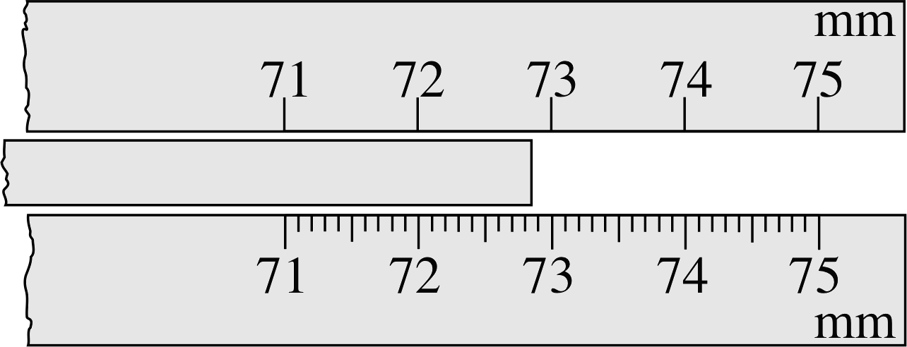
Figure 1 Two scales being used to measure the length of a rod. The top scale can be read only to within 0.1 mm at best, but you may feel that you can read the bottom scale to within 0.02 mm.
You are therefore claiming an uncertainty of ±0.05 mm i, and you should quote your result as (72.8 ± 0.05) mm. Using the bottom scale in Figure 1, you can probably read the result with an uncertainty of ±0.03 mm; if so, you would be justified in recording your answer as (72.86 ± 0.03) mm. Be careful, though, not to claim a level of precision that you cannot really achieve, especially when you have to judge fractions of a scale division.
Even if no uncertainty is explicitly given, it is implicit in the number of figures quoted in the result – so it would be incorrect to claim that the length was (say) 72.8516 mm unless you had a scale with much finer divisions and a way of reading it that precisely.
These are examples of an extremely important general rule:
Never quote a result to more figures than you can justify in terms of the uncertainty of your measurement.
The meaningful digits (i.e. individual figures) that appear in the value of a physical quantity and which indicate its precision are usually referred to as significant figures.
The lengths 82.5 mm and 0.0825 m are both said to be known to three significant figures, even though in the latter case an extra zero is essential to fix the location of the first non–zero digit relative to the decimal point. Thus, the significant figures in a quantity do not include any zeros to the left of the first non–zero digit.
Zeros at the end of a number may or may not be significant. For instance, if you state that a length is 82.50 mm you really should mean that the length is known to the nearest 0.01 mm and that the final zero is significant. However, if you were asked to express 82.5 mm in terms of micrometres (μm) you might be tempted to write 82500 μm even though you know the final zeros are not significant. Of course, anyone else reading this number would have no way of telling whether the final zeros were significant or not. Thus zeros at the end of a whole number are ambiguous, they may or may not be significant.
✦ How can you avoid writing down zeros at the end of a whole number when you know they are not significant?
✧ Use scientific notation. A value such as 82.5 mm can be written as 8.25 × 104 μm without introducing spurious zeros.
So, to summarize:
The significant figures in a number are the meaningful digits that indicate its precision. They do not include any zeros to the left of the first non–zero digit. Using scientific notation avoids the need to write down any zeros that are not significant, either to the right or the left of the significant figures.
If your calculator displays the result of a calculation as 2.0375, you could write this as
2 (to one significant figure)
2.0 (to two significant figures)
2.04 (to three significant figures)
2.038 (to four significant figures)
Note the convention: If the last significant figure had been followed by a number from 0 to 4, it would have been unchanged, but if it had been followed by a number from 5 to 9, the last significant figure would have increased by one. This process is called rounding. When the last digit is increased we say the value has been rounded up, and when the last digit is left unchanged the value is said to have been rounded down.
Question T7
Express the following in scientific notation to three significant figures:
(a) 128 456.1 (b) 0.015 446 69 (c) 0.002 6991
Answer T7
(a) 1.28 × 10⁵
(b) 1.54 × 10⁻²
(c) –2.70 × 10⁻³
Significant figures are particularly important in calculations in which measured values are combined. The reason for this is easy to understand. If you know that a length l1 = 3.28 m (implying that it lies between 3.275 m and 3.285 m) and that a length l2 = 0.0524 m, you might be tempted to say that l1 + l2 = 3.3324 m. However, this would be very misleading since it seems to indicate that the uncertainty in l1 + l2 is ±0.000 05 m whereas, due to the large uncertainty in l1, the uncertainty in l1 + l2 is really more like ±0.005 m. By restricting the number of significant figures in an answer to the number of significant figures in the quantities used to obtain that answer you will avoid this problem.
When multiplying or dividing two numbers, the result should not be quoted to more significant figures than the least precisely determined number. (So, 0.4 × 1.21 = 0.5)
When adding or subtracting two numbers, the last significant figure in the result should be the last significant figure that appears in both the numbers when they are expressed in decimal form without powers of ten. (So, 0.4 + 1.21 = 1.6 and 0.004 + 1.21 = 1.21)
Finally, note that many calculations involve accurately known quantities such as the numerical constant π (= 3.141 592 65 to nine significant figures) or whole numbers such as 2, 3, 4, 5, etc. Since these quantities are so precisely known they should not usually limit the number of significant figures in an answer.
Question T8
Calculate each of the following to three significant figures, rounding as appropriate: i
(a) 10/3 (b) 7 × 321 (c) 100/11 (d) (4.23 × 10⁻²/(3 × 10−4)
Answer T8
(a) 10/3 = 3.333 33... = 3.33 to three significant figures.
(b) 7 × 321 = 2247 = 2.247 × 103 = 2.25 × 10³ to three significant figures.
(c) 100/11 = 9.090 909... = 9.09 to three significant figures.
(d) 1.41 × 10² to three significant figures.
4.2 The importance of errors
When physicists present the results of experimental measurements, they nearly always specify a possible error associated with the quoted results. Used in this context the word ‘error’ has a very specific meaning. It does not mean that the scientist made a mistake when doing the experiment; what it does mean is that – because of the inherent limitations of the equipment or of the measurement techniques – there will be some uncertainty associated with the final result. Thus ‘error’ is synonymous with ‘uncertainty’ and is indicated in the same way. For example, a result can be expressed in the form (50 ± 3) seconds; this is read as ‘50 plus or minus 3 seconds’. This means that your best estimate of the result is 50 seconds, but it could be as low as 47 seconds or as high as 53 seconds. The answer is uncertain by plus or minus 3 seconds – this represents the error in this case.
Here are some examples to show why error estimates are important:
✦ A theory predicts that about 7.0 MeV i of energy will be released in a certain nuclear reaction. When the experiment is carried out, an energy release of 6.5 MeV is observed. Does the experiment disprove the theory?
✧ Not necessarily; we have to ask what are the errors in both the experimental and theoretical values. If the error in each was ±0.5 MeV, then theory and experiment would be quite consistent, but if the errors were only ±0.1 MeV, then the theory or the experiment or both should be called into question. So the same result could lead to different conclusions, depending on the size of the error.
✦ Two experimenters measure the period of a pendulum. One quotes the result as (2.04 ± 0.03) s and the other as (1.94 ± 0.08) s. In which result would you have most confidence?
✧ Obviously, the first. The quoted error is less than half that obtained by the second experimenter, which indicates a more precise measurement. We assume of course that the errors quoted are realistic!
Question T9
(a) Are the results obtained by the two experimenters in the above question consistent?
(b) Suppose the errors had both been ±0.03 s. Would your answer to (a) be any different ?
Answer T9
(a) The first experimenter’s result could have been as low as 2.01 s (2.04 s − 0.03 s), and the second experimenter’s result could have been as high as 2.02 s (1.94 s + 0.08 s). These overlap, so the results are not inconsistent.
(b) If the errors were both ±0.03 s, the lower limit on the result from the first experimenter could have been higher than the upper limit on the result from the second experimenter; so in this case the results are not consistent. (The lesson to be learned here is that before we make comparisons between the results obtained by two or more experimenters, we must have good estimates of the error in each case.)
4.3 How do errors arise?
Mistakes! First, let us dispose of human errors that are just silly blunders: misreading a scale, adding up the values on a scale wrongly, recording a number wrongly, or making a mistake in the calculation. These are not really errors in the scientific sense at all. The best advice we can give you is ‘don’t make them!’ Fortunately, mistakes like this generally show up if the measurements are repeated, and certainly all of them can be avoided by taking more care and checking whenever possible.
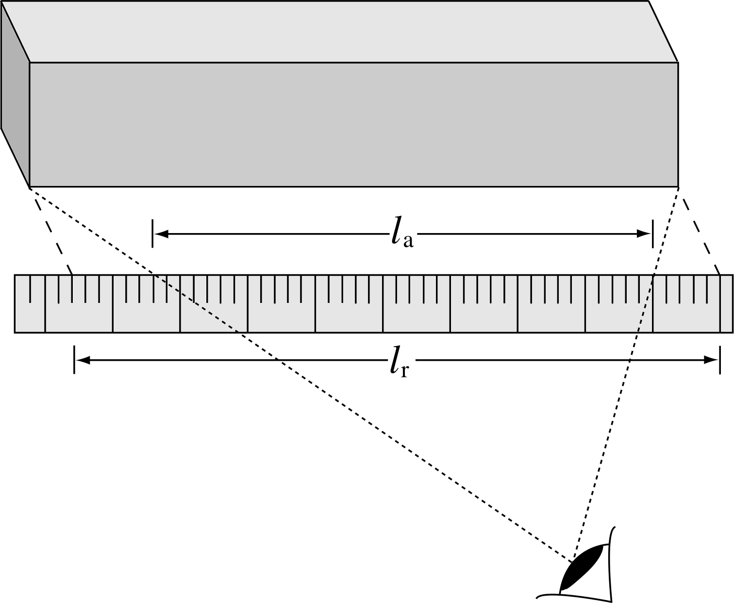
Figure 2 Parallax errors arising in the measurement of the length of an object. The apparent length, la in this case, is shorter than the real length lr, which would be measured if the scale were placed in contact with the object.
Human errors For example, parallax errors (illustrated in Figure 2), misaligning a measuring instrument or simply not setting it up as accurately as possible. Some of these errors can be avoided by using digital instruments, where numbers are displayed directly rather than being read from a scale by an observer.
Instrumental error All measuring instruments have their limitations. Some are obvious (e.g. unequal spacings on a cheap wooden scale); others are not so apparent.
However, even the most expensive and sophisticated instrument will only be capable of being used to a certain precision. With a digital instrument, a reading precision of ±1/2 of the last significant figure is the best that can be achieved. For an instrument with a scale and pointer, the reading precision will be determined partly by the fineness of the scale divisions, and partly by how well the observer can judge readings between scale divisions. Another important source of instrumental error arises from imperfect instruments, for example, friction in the balancing mechanism of an instrument or a lack of reproducibility due to construction limitations.
Errors caused by the act of observation For example, connecting a pressure gauge to a tyre causes a small drop in pressure, and a hot liquid cools slightly when a cold thermometer is immersed in it.
Errors caused by extraneous influences A variety of unwanted effects can cause errors in experiments. Draughts lead to errors when weighing with a sensitive balance, while changes of temperature can lead to errors in many different experiments. Attempts should always be made to eliminate these effects, or at least to reduce them.
In the preceding discussion we have assumed that the quantity we are trying to measure has a well defined value, and that our aim is to find this value as precisely as possible, e.g. the length of a table, the mass of a booklet, and so on.
However, quite a number of measurements attempt to quantify something that is not fixed, e.g. the lifetime of a given type of radioactive nucleus or the mass of an adult. In such cases we have to turn to the field of statistics – the branch of mathematics that deals with the study of numerical data and the inferences that can be drawn from such data. When faced with a number of nuclear lifetime measurements or a list of masses of adults the statistical quantity that is most often required is the mean or average of the data.
The mean of n values of a quantity a (i.e. the mean of a1, a2, a3, a4, ... an−2, an−1, an) is symbolized by $\langle a \rangle$ i and is defined by
$\displaystyle \langle a \rangle = \dfrac{a_1+a_2+a_3+a_4+\ldots+a_{n-2}+a_{n-1}+a_n}{n} = \dfrac{1}{n}\sum_{i=1}^n a_i$
where the summation sign $\sum$ indicates that whatever follows is to be summed for all values of i between 1 and n. i
Mean values determined from a set of measurements are subject to two additional sorts of error: those due to statistical fluctuations, and those due to unrepresentative samples.
Errors due to statistical fluctuations When we make measurements on a sample drawn from a large population, i and try to deduce average properties of the population from these measurements, then we are likely to introduce errors. For example, suppose we measured the heights of ten men aged 30 in a certain city. We would find a range of values for the height and could calculate the mean. If we repeated the experiment with another sample of ten men aged 30, the average height would most likely be different. So, although measurements on a sample of ten men give us an estimate of what the average height of all 30-year-old men is, it cannot be a precise result – there must be some uncertainty, some error associated with the fact that we have only taken a limited sample. As you might expect, the error in the estimate of the mean height gets smaller as the size of the sample grows, but there will always be some statistical uncertainty as long as we are only measuring a selection from the complete population.
Errors due to use of unrepresentative samples It is essential, when using a sample of measurements to deduce properties of a larger population, that the sample chosen is typical of the complete population. Continuing our example above, if we wanted to know the average height of all men aged 30 in our chosen city, then it would be a mistake only to measure (say) members of the rugby club!
4.4 Random and systematic errors
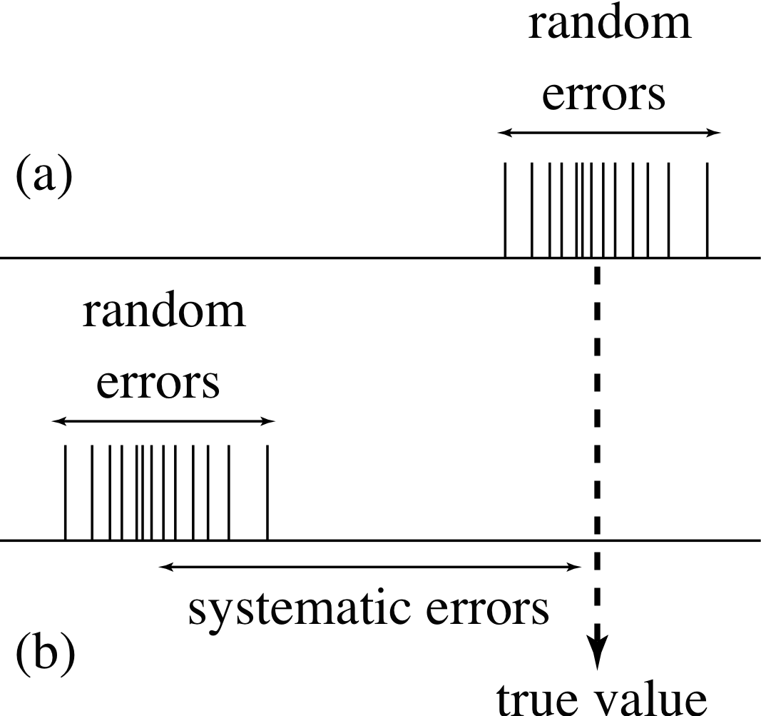
Figure 3 (a) Random errors alone lead to a spread of measurements about the true value. (b) Systematic errors lead to a displacement of the measurements, and when random errors are present as well, the measurements are not spread about the true value.
Some of the sources of error discussed in Subsection 4.3 give rise to random errors – they are equally likely to produce results above or below the true value. Averaging a number of readings tends to cancel out the effects of such errors, and (as will be discussed in more detail in Subsection 4.5) the spread of the readings allows us to estimate the size of the random errors involved. Unfortunately there are other types of error – known as systematic errors – which systematically shift the measurements in one direction away from the true value. Repeated readings do not show up the presence of systematic errors, and no amount of averaging will reduce their effects. However, if a there is a known systematic error in a measurement it is often possible to eliminate its effect. For example, if we know that rugby players are on average 10 cm taller than non–rugby players we could correct for it in our predictions. Both systematic and random errors are often present in the same measurement, and the different effects they have are contrasted in Figure 3.
Random errors lead to a spread of measurements about a mean value. Systematic errors lead to a displacement of the mean value from the true value. The accuracy of a measurement, refers to its difference from the true value, and is determined by both the random and the systematic errors involved in that measurement. The precision of a measurement refers to its sensitivity and agreement with similar measurements, and is determined only by the random errors. Eliminating sources of systematic error makes a precise measurement more accurate.
Many systematic errors arise from the measuring instrument used. For example, a metre rule may in fact be 1.005 m long, so that all measurements made with it are systematically 0.5% too short. Or the ruler may have 0.1 mm worn from one end, so that all lengths measured systematically appear 0.1 mm longer than they are. In general the accuracy of an instrument is specified by its manufacturer. Before releasing a piece of equipment the manufacturer checks it against another, more accurate one. This process is called calibration. The manufacturer may say that the specified accuracy will only be obtained under certain conditions; for example, a metal scale may be calibrated at 20°C, so that it becomes less accurate as the temperature deviates from 20 °C, owing to the expansion or contraction of the metal. Systematic errors in instruments can often only be discovered and estimated by comparison with a more accurate and reliable instrument (i.e. during calibration) and so the instrument should be recalibrated wherever possible. If this is done, the effects of these errors can be reduced by correcting the measured results.
The experimenter may also introduce errors into the experiment, both random and systematic. The small but finite time that an experimenter takes to react to a given situation could be a source of systematic error in any experiment that depended on measuring the time at which a particular event occurred. On the other hand, in an experiment that involved measuring the duration of an interval (such as the time required for a pendulum to swing back and forth), the systematic effects of the experimenter’s reaction time at the beginning and end of the interval might well cancel, but his or her random errors would still remain.
Question T10
Of the sources of error discussed in Subsections 4.3 and 4.4, identify at least two that would give rise to systematic error.
Answer T10
Sources of systematic error may include: instrumental error (e.g. if a metal ruler calibrated at 20°C is used at 25°C, it will have expanded and so all readings will be systematically low); error caused by the act of observation (e.g. connecting a pressure gauge will always cause a slight drop in the pressure that is being measured); error due to the use of unrepresentative samples (e.g. measuring the heights of rugby players will give a systematic overestimate of the average height of people in general).
4.5 Estimating the size of random errors
Often one of the most difficult parts of an experiment is the estimation of the size of the random errors involved. Obviously, no two experiments are exactly alike, so it is impossible to give hard and fast rules about how this should be done. However, we will suggest an approach to this problem which you can use in most circumstances.
Determine whether or not the result is reproducible
The first thing to ascertain is whether a measured value is reproducible. Usually, you should not be satisfied with a single measurement: repeat the measurement several times if possible. And, usually, you should reset the measuring instrument each time. If you are measuring the length of a rod, remove the ruler, reposition it, and read off the length again. When measuring the mean diameter of a wire with a gauge, remove the gauge and reposition it to a different point on the circumference of the wire before taking another measurement. Notice that a major factor here is the uncertainty in setting the position, and this is often much larger than the uncertainty in reading the scale itself.
If the result is not reproducible ...
In most cases (though not all), you will find that repeating measurements produces different results. This is because of the random variations in the way that measuring instruments are set up; random variations in the judgement of the scale reading; random variations in the quantity actually being measured; and so on. All measurements are subject to such random errors. The random error associated with any measurement determines the variability of the results, and the questions to ask are: what is the best value of the quantity measured, and how do we estimate an error from the variability?
As an example, consider an experiment in which five measurements are made of the rate of flow of water from a tap. In particular, suppose that the volumes of water collected in five periods of four minutes are 436.5 cm3, 437.5 cm3, 435.9 cm3, 436.2 cm3 and 436.9 cm3.
Assuming that there is nothing to choose between these measurements (i.e. they were all taken with the same care and skill, and with the same measuring instruments), then the best estimate of the volume V of water supplied in four minutes is the mean value $\langle V \rangle$ i of the five readings, and we can write
V = $\langle V \rangle$ = (436.5 + 437.5 + 435.9 + 436.2 + 436.9) cm3/5 = 436.6 cm3
When several equally good measurements of a quantity are available, the best estimate is provided by the mean of the measurements.
What error should we associate with this mean value? The measurements are spread out between 435.9 cm3 and 437.5 cm3, that is from (436.6 − 0.7) cm3 to (436.6 + 0.9) cm3. If we average the negative and positive deviations from the mean, then we can say that the spread is about ±0.8 cm3. However, the volume is unlikely to lie right at the ends of this range, so quoting an error as ±0.8 cm3 would be unduly pessimistic. It is more realistic to apply the following rule of thumb.
As a rough rule of thumb, when several equally good measurements give a spread about a mean value, the random error may be taken to be about 2/3 of the spread. i
So in this case the error is about ±0.5 cm3. Note that this only a rough rule of thumb, and it still overestimates the error in the mean value, particularly when a large number of measurements are taken.
Obviously, if one reading were very different from all of the others, then a determination of the likely error from the spread would be misleadingly pessimistic. Common sense usually suggests that the odd reading is ignored when calculating the mean and the error, and that a few more measurements are taken. i For example, if the last reading for the volume were 432.9 cm3 rather than 436.9 cm3, then it would be wise to repeat it.
In the example we have just discussed, the variability in the measured values of V could arise from the combination of a number of factors. These include actual variations in the flow rate, errors in timing the four–minute periods, inserting and removing the beaker to collect the water too early or too late, and inaccuracies in measuring the volume collected. The beauty of repeating measurements is that we get an overall measure of the random errors involved, and it isn’t necessary to assess the individual contributions.
Question T11
The masses of 20 male marmoset monkeys were obtained as part of a study on the growth of marmosets. The masses in grams (g) of the 20 individuals at six days after birth were as follows: 280, 275, 283, 264, 272, 280, 290, 287, 283, 276, 278, 282, 280, 288, 282, 265, 291, 282, 279, 278. Make a rough estimate of the random error in these measurements.
Answer T11
The mean value is 280 g. (If you thought it was 279.75 g you were deluding yourself, there was no justification for five significant figures.) The largest reading is 291 g, which is 11 g above the mean, and the lowest reading is 264 g, which is 16 g below the mean. The average of 11 g and 16 g is 13.5 g. Thus the estimate of error is 2/3 × 13.5 g = 9 g and the result could be quoted as (280 ± 9) g.
(Of course, this is just a crude estimate of the error. More precise methods are discussed elsewhere in FLAP.)
If the result is reproducible ...
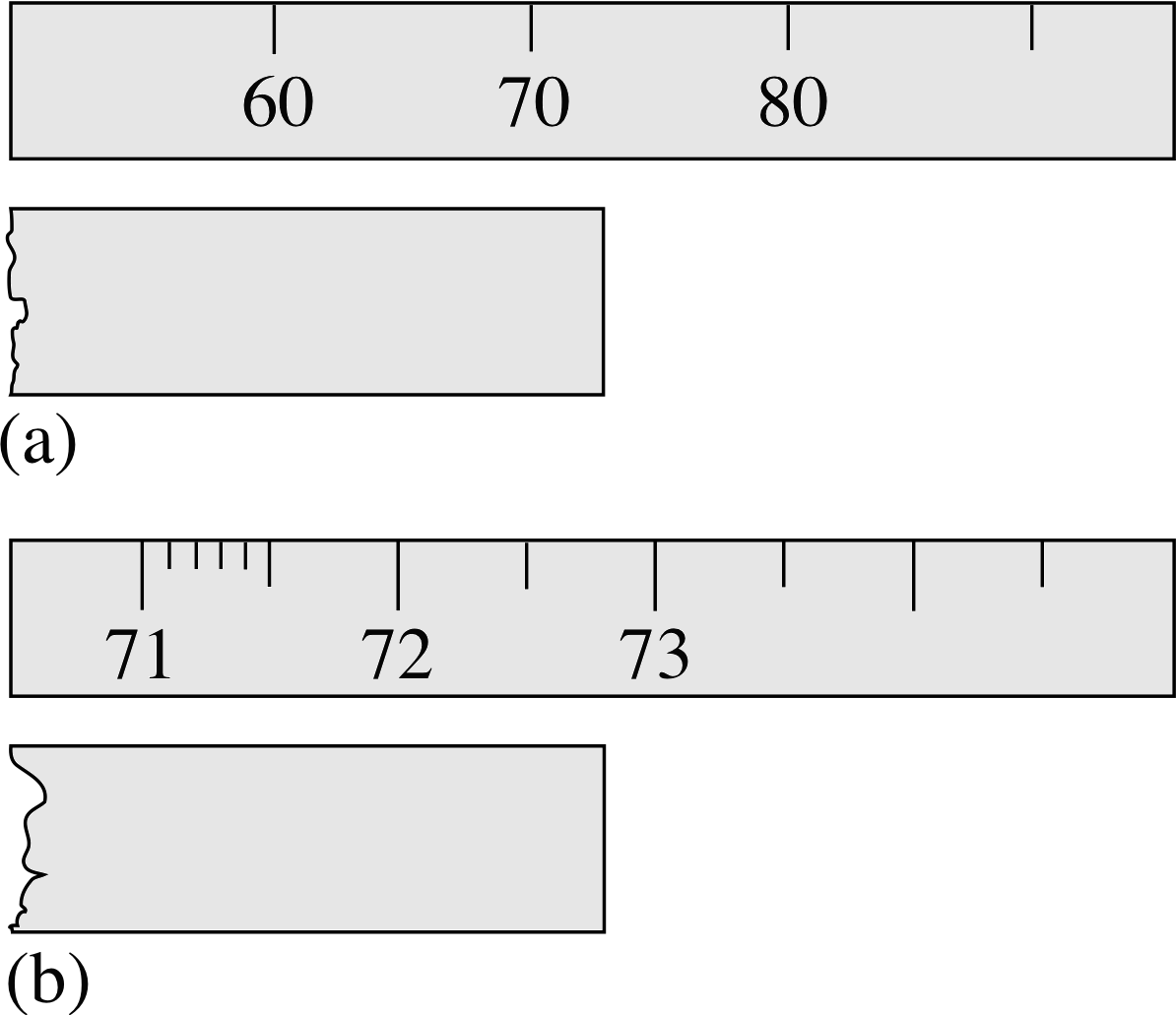
Figure 4 The scale in (a) can be read to the nearest 1 mm, but the scale in (b) to the nearest 0.1 mm. (Note that the scales are shown without units in this figure.)
You will find when repeating some experimental measurements that you record exactly the same result each time. Does this mean that there is no error associated with the measurement? In most cases, it certainly does not. To take a simple example again, assume that the results of measuring the length of a bar five times were: 73 mm, 73 mm, 73 mm, 73 mm and 73 mm, i.e. five identical readings. Here we can deduce the error from the number of significant figures recorded. By writing down 73 mm, the experimenter is implicitly recording that the length is closer to 73 mm than it is to 72 mm or to 74 mm, or that the length lies between 72.5 mm and 73.5 mm. The error is therefore ±0.5 mm, and the result should be quoted as (73 ± 0.5) mm. Of course, this uncertainty has resulted from the limitations of the measuring equipment. One of the first things you should do when you use a piece of equipment is assess the inherent limitations of the equipment itself.
Naturally, in situations such as this, where identical readings are obtained, it is particularly important to make sure that you are reading the instrument as precisely as possible. With the scale shown in Figure 4a, the quoted results are the best that can be expected. However, the scale shown in Figure 4b can be read more accurately – a value of 72.8 mm could be recorded in this case. A set of repeated measurements might then show some variability from which the likely error could be deduced. Of course, if repeated measurements all came up with the result 72.8 mm, then we would have to conclude that the error was ± 0.05 mm.
Question T12
An experimenter is using a balance that gives a reading that is accurate to the nearest 1 mg. The mass of a certain crystal is recorded as 170 mg. How should the experimenter quote the result of this mass determination?
Answer T12
Crystal mass = 170 ± 0.5 mg. Alternatively, using scientific notation this could be expressed as 1.70 × 10² mg where the final zero is significant and the uncertainty is ±0.5 mg.
In all the examples we have given so far, the errors have been quoted as actual values, e.g. ±0.05 mm, ±0.8 cm3, etc. Such errors are called absolute errors. However, it is sometimes useful to express an error as a fraction of the measurement itself; errors expressed in this way are called fractional errors. For example, in the case of the length measurement discussed at the start of Subsection 4.1:
absolute error = 0.05 mm, measurement = 72.8 mm so, fractional error = 0.05 mm/72.8 mm = 0.0007
Note that we have only given the fractional error to one significant figure, because the original absolute error was only given to one significant figure.
More commonly, the fractional error is multiplied by 100% to give the percentage error. In the above example: percentage error = (0.05 mm/72.8 mm) × 100% = 0.07% i
Question T13
Express the error given in Question T12 as a fractional error and a percentage error.
Answer T13
Fractional error = 0.5/170 = 0.003.
Percentage error = (0.5/170) × 100% = 0.3%.
(Note that the errors are quoted to one significant figure in each case, because the original absolute error is quoted to one significant figure.)
5 Errors in the counting of randomly–occurring events
5.1 Errors due to sampling
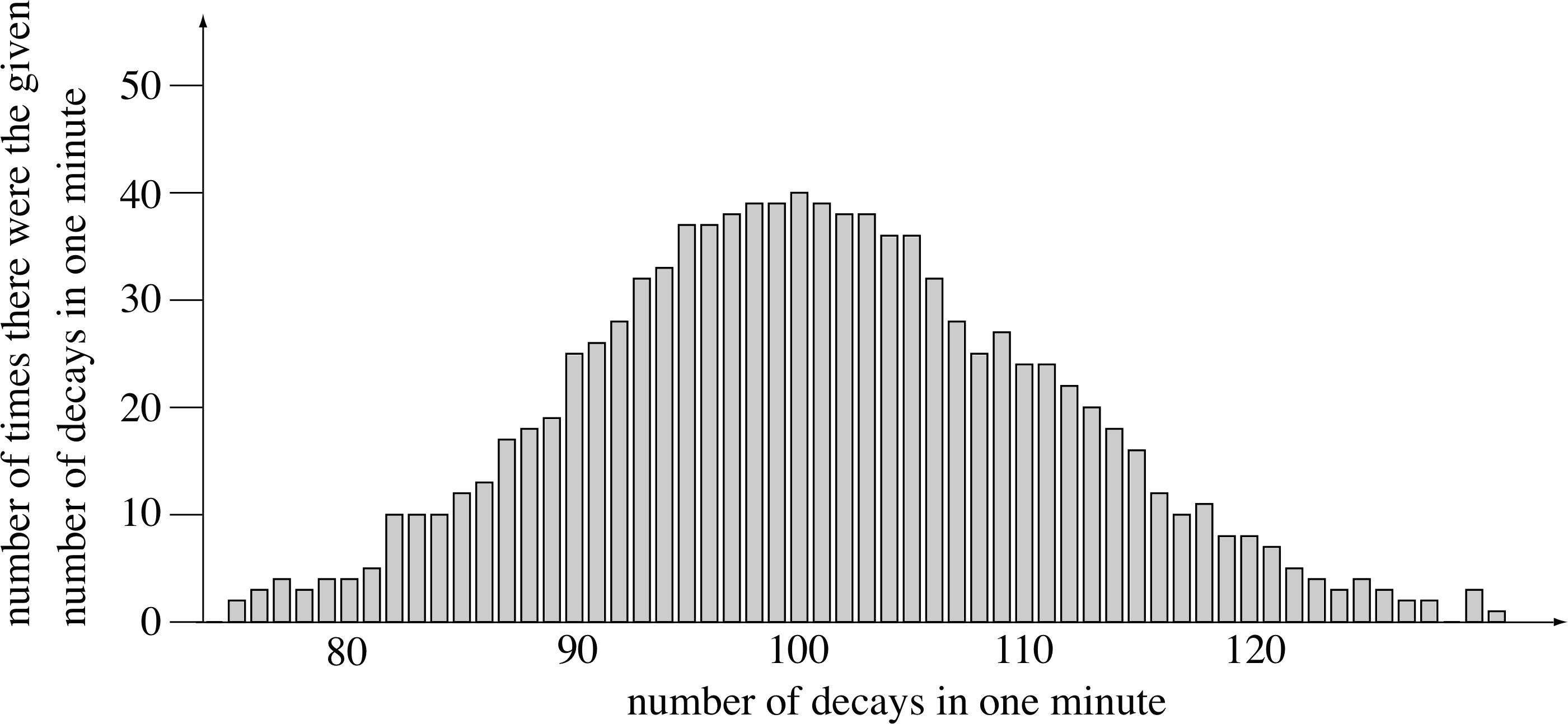
Figure 5 The distribution of the number of radioactive decays (between 74 and 129) that occurred in 1000 counting periods of 1 min.
In Subsection 4.3, your attention was drawn to the error that resulted from calculating a mean value for a quantity when only a sample of the whole population was considered. There, we quoted, as an example, the estimation of the mean height of a population of 30-year-old men from a random sample of just ten such men.
The problem we discuss in this section is that of estimating the error that is likely to arise from such sampling procedures.
A good example is an experiment that involves the determination of the number of nuclei decaying each minute in a radioactive pellet. Suppose that you observed 107 decays in the first minute. How many would you observe in the second minute? You might expect to record the same number, 107, but that is unlikely since each decay is an event occurring at a random time, and therefore there is no reason to expect the total number of such random events in a given period to be constant. However, it would be quite reasonable to expect that in a pellet containing a large number of nuclei, the statistical variations would partially cancel each other out so that the number of decays in each minute would be about the same. In fact, if you performed the experiment 1000 times you might well find that the number of decays per minute varied as in Figure 5.
The mean result of the 1000 experiments is 100 decays per minute. i But the distribution shows that counts as high as 110 and as low as 90 occur with reasonable frequency. In fact, if the mean is 100 counts, about two–thirds (actually 68%) of experiments have a result between 90 and 110 counts, or within ±10 counts of the mean. (You may have noticed that 10 is one of the square roots of 100, the mean value – the significance of this is explained below.)
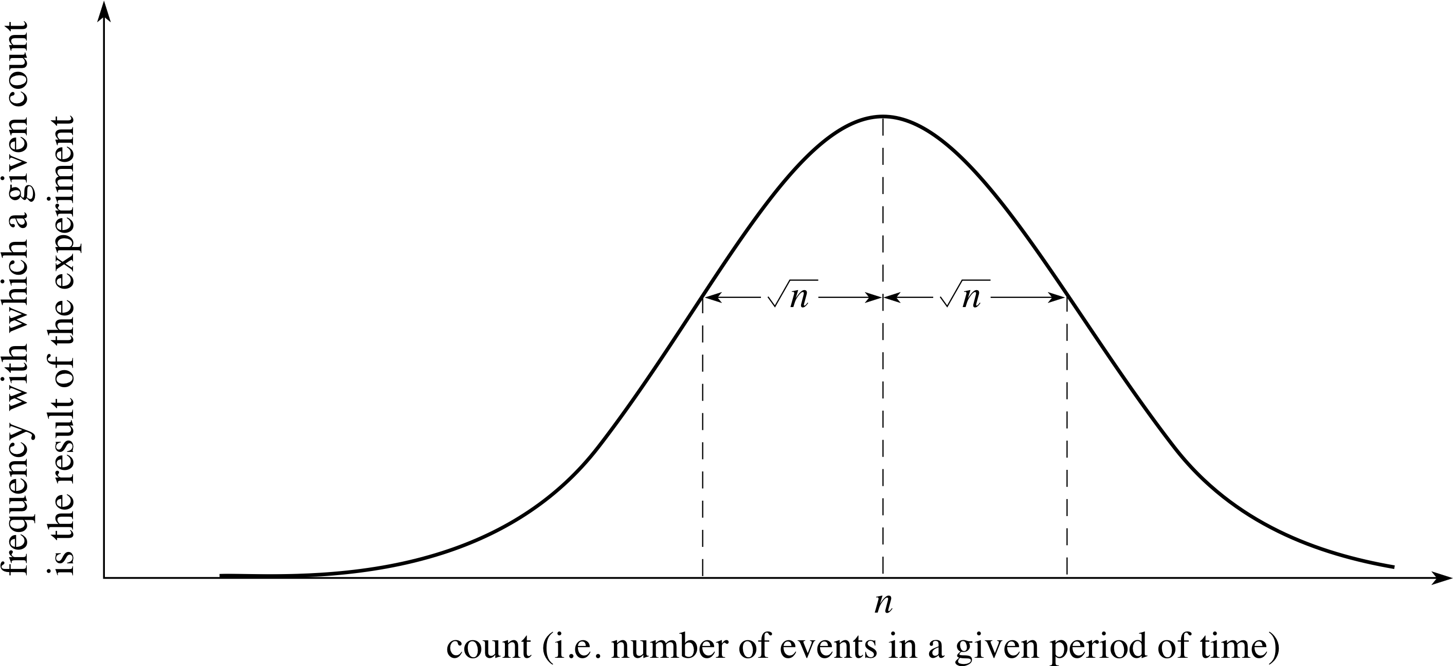
Figure 6 The result of a very large number of identical experiments to determine the number of times a randomly–occurring event takes place in a given period of time (i.e. its frequency). The mean n is at the peak of the distribution and 68% of all the readings are within ±n of this mean.
In general, if a determination is made of the number of times a randomly–occurring event takes place in a given period of time and the experiment is repeated over and over again, the distribution of results will tend, as the number of experiments increases, to the curve shown in Figure 6. It turns out that 68% of the experiments will give a result within ± n of the mean.
The quantity n is therefore a convenient way of characterizing the distribution, and can be used as a measure of the uncertainty in the number of events counted. So if the mean is 100 counts, 68% of the experiments will produce a result between 90 and 110 counts. Or, if the mean is 900 counts, the corresponding values defining the width of the distribution are 870 and 930. It follows from this argument that we can easily identify the uncertainty or error associated with a single counting experiment.
In a single counting experiment, if the number of randomly–occurring events counted in a given period is N, the uncertainty in this count (i.e. the likely difference between N and the mean that would be found from repeated experiments) is $\sqrt{N\os}$.
In the example above, the fractional error in a single measurement of 100 counts would be 10/100 = 0.1, and that in a single measurement of 900 counts would be 30/900 = 0.03. So the N rule points to the desirability of counting over a long period, i.e. taking a large sample. Therefore we can deduce that increasing the number of counts reduces the fractional error, i.e.
$\text{fractional error} = \dfrac{\text{error}}{\text{value}} = \dfrac{\sqrt{N\os}}{N} = \dfrac{1}{\sqrt{N\os}}$
Unfortunately, as the answer to Question T15 (below) shows, the rate at which the fractional error falls with increasing N is frustratingly slow.
One of the skills every experimentalist must learn is that of balancing the time invested in an experiment against the accuracy of the result.
Question T14
A radioactive sample has an mean activity of 100 decays per minute. In any given minute, what is the chance of getting more than 110 decays? (Express your answer as a percentage.)
Answer T14
If we make a series of one minute counts, about 68% of them will be between 90 and 110 (100 ± 10). So about 32% will be outside this range. Since the distribution is symmetrical, about 16% will be above 110.
Question T15
A radioactive sample has an mean activity of 100 counts per minute.
(a) Approximately how long would it take to produce 900 counts (i.e. to take a single measurement with a fractional error of 0.03)?
(b) In order to reduce the fractional error in a single measurement to 0.01, how many counts would need to be recorded? Approximately how long would this measurement take?
(c) By how much is it necessary to increase the sampling time T to reduce the fractional error in a measurement from e to e/x, where x is a number greater than 1?
Answer T15
(a) 9 minutes.
(b) If the fractional error $1/\sqrt{N\os} = 0.01$, then, N = 100 and hence the number of counts to be recorded would be N = 104. At an average activity of 100 counts per minute, it would take approximately 100 minutes to produce this many counts.
(c) To reduce $1/\sqrt{N\os}$ by a factor of 1/x, to $1/(x\sqrt{N\os})=1/\sqrt{x^2N}$, the count must be increased from N to x2N, so the sampling time must also be increased by a factor x2 from T to x2T.
6 Closing items
6.1 Module summary
- 1
-
It is important to have well–defined units and precise, reproducible standards of measurement. In the metric system of SI units, the Subsection 2.3basic units of length, mass and time are the metre, kilogram and second.
- 2
-
A particular quantity may be expressed in a variety of units, which may be converted from one into another and which all have the same dimensions.
- 3
-
Subsection 3.1Dimensional analysis can be used to test the validity of equations. An equation must be false if it equates, adds or subtracts quantities with different dimensions.
- 4
-
When recording experimental data, it is important to quote an appropriate number of significant figures. It is also very important to give an estimate of the Subsection 4.2error or uncertainty in any measurements or results.
- 5
-
The precision of a measurement concerns the sensitivity and reproducibility of the determination. The accuracy of a measurement concerns the departure of the measurement from the true value.
- 6
-
Random errors are equally likely to make the measurement high or low but systematic errors introduce a bias of the measurement away from the true value. Precision is affected only by random errors but accuracy is affected by systematic errors as well as by random errors.
- 7
-
Random errors may be estimated by taking several readings, working out their mean, and examining the spread of the readings around that mean. (The random error is roughly 2/3 of the spread.)
- 8
-
systematic errorsSystematic errors are harder to estimate and generally have to be determined by performing a more accurate experiment.
- 9
-
The uncertainty in a measurement or result may be expressed as an absolute error, a fractional error or a percentage error.
- 10
-
The uncertainty in the number of random events occurring in a given period of time (e.g. radioactive decays) is equal to the square root of the mean number of those events. The percentage errorpercentage uncertainty can be reduced by increasing the period of time.
6.2 Achievements
Having completed this module, you should be able to:
- A1
-
Define the terms that are emboldened and flagged in the margins of the module.
- A2
-
Explain the importance of well–defined and reproducible units.
- A3
-
Explain how the basic units of the Système International d’Unités are defined.
- A4
-
Convert quantities expressed in terms of one unit into quantities expressed in terms of another unit.
- A5
-
Explain the difference between units and dimensions and determine the dimensions of a quantity given its units.
- A6
-
Use dimensional analysis to check the consistency of formulae.
- A7
-
Express a given result to a specified number of significant figures, and explain why this might be necessary.
- A8
-
Explain the importance of experimental errors, and describe some of the ways in which errors can arise.
- A9
-
Distinguish between random and systematic errors, and between precision and accuracy. Explain how these errors can be estimated, and perform simple error estimates given appropriate results.
- A10
-
Estimate the error in a mean number of randomly–occurring events.
Study comment You may now wish to take the Exit test for this module which tests these Achievements. If you prefer to study the module further before taking this test then return to the topModule contents to review some of the topics.
6.3 Exit test
Study comment Having completed this module, you should be able to answer the following questions each of which tests one or more of the Achievements.
Question E1 (A2)
Explain why, in science, standards of mass, length and time must be agreed internationally.
Answer E1
Modern scientific research involves cooperation between scientists and laboratories all over the world. Scientists could not begin to communicate their results to each other if they did not agree on the units!
(Reread Subsections 2.1 and 2.2 if you had difficulty with this question.)
Question E2 (A3)
Describe one important difference between the definition of the SI unit of mass and the definitions of the units of length and time.
Answer E2
The SI units of length and time are defined with reference to atomic standards - the wavelength of krypton light and the frequency of the vibration of caesium atoms, respectively. (The definition of the unit of length is further refined by using the definition of the second and defining the speed of light in a vacuum to have a fixed value.) In contrast, the SI unit of mass is based on the mass of a cylinder of platinum-iridium. There is as yet no atomic standard of mass which is sufficiently precise to be used for everyday mass comparisons.
(Reread Subsection 2.2 if you had difficulty with this question.)
Question E3 (A4)
The radius of the Sun is 6.96 × 10⁵ km. Express this distance in miles, using the conversion factor 1 mile = 1.609 km.
Answer E3
6.96 × 10⁵ km = 6.96 × 105 km × (1 mile/1.609 km) = (6.96 × 10⁵/1.609) miles = 4.33 × 10⁵ miles.
(Reread Subsection 2.4 if you had difficulty with this question.)
Question E4 (A3 and A5)
Classify the terms below into the following categories:
(a) SI basic unit
(b) SI derived unit
(c) SI basic unit multiplied by a power of ten
(d) SI derived unit multiplied by a power of ten
(e) other units
(f) dimensions.
centimetre, mass, mile, kHz, kelvin, GW, length, kg, henry, hertz, mmol, acre.
Answer E4
(a) kelvin, kg
(b) henry, hertz
(c) centimetre, mmol
(d) kHz, GW
(e) mile, acre
(f) mass, length
(Reread Subsections 2.2, 2.3, 2.4 and 3.1 if you had difficulty with this question.)
Question E5 (A6)
An object moves with constant speed υ in a circle of radius r. The magnitude a of its acceleration is claimed to be given by a = 2υ2/r. Is this equation dimensionally consistent?
Answer E5
Dimensions of a are L T−2. Dimensions of υ are L T−1, so υ2 has dimensions L2 T−2. Dimensions of r are L. Dimensions of υ2/r are L2 T−2/L = L T−2, the same as those of a, so the equation is dimensionally consistent. In fact, a = υ2/r, so the equation is wrong even though it is dimensionally consistent.
(Reread Subsection 3.1 if you had difficulty with this question.)
Question E6 (A7)
Evaluate the following: (2.998 × 2.022 × 10−22)/[(2.107 × 10−22) × (1.75 − 0.74)].
Express your answer in scientific notation to two significant figures.
Answer E6
2.8.
Note that the rounding of the last significant digit is determined by the digit immediately to its right and has nothing to do with any of the later figures.
(Reread Subsection 4.1 if you had difficulty with this question.)
Question E7 (A8)
You are handed a stopwatch and a pendulum (a piece of string with a weight on the end) which is one metre in length. You are then asked to find the period of swing of the pendulum. What are the main sources of random and systematic error likely to be?
Answer E7
The main sources of random error are likely to be in deciding when a swing starts and finishes, and in reading the stopwatch scale.
Errors in starting and stopping the watch may be random, although there could be a systematic error here too – always starting the watch too late, for example. If the watch runs consistently slow or fast, this will give rise to a systematic error.
(Reread Subsections 4.3 and 4.4 if you had difficulty with this question.)
Question E8 (A9)
Ten measurements of the period of the pendulum described in Question E7 were as follows:
2.13 s, 32.07 s, 32.24 s, 32.20 s, 32.08 s, 32.11 s, 32.15 s, 32.19 s, 32.22 s, 32.16 s
What is the mean value of the period? What is the random error?
Answer E8
Mean value of period = 2.16 s.
Highest reading is 2.24 s, i.e. 0.08 s above the average value.
Lowest reading is 2.07 s, i.e. 0.09 s below the average value.
So the random error is approximately ±0.09 × 2/3 = ±0.06 s.
(Reread Subsection 4.5 if you had difficulty with this question.)
Question E9 (A9)
If the length l of the pendulum described in Question E7 is exactly one metre, and the period T is given by $T=2\pi\sqrt{l/g}$ what is the approximate systematic error in the timings given in Question E8? (Take g = 9.81 m s−2).
Answer E9
Given that l = 1 m and g = 9.8 m s−2, it follows from the formula that T = 2.01 s. So the systematic error is equal to 2.16 s – 2.01 s = 0.15 s.
(Reread Subsections 4.4 and 4.5 if you had difficulty with this question.)
Question E10 (A10)
A certain radioactive sample has on average 250 decays per minute. For how many minutes must counts be carried out to obtain this rate with a percentage error of 1%?
Answer E10
If a sample is counted for n minutes, the number of counts will be about 250n and the uncertainty in this number of counts will be approximately $\sqrt{250n\os}$.
So, if the percentage uncertainty is 1%,
$\left(\sqrt{250n\os} \times 100\%\right)/(250n) = 1\%, \;\text{i.e.}\; 100 = \sqrt{250n\os}$
Thus, 10 000 = 250n, i.e. n = 40.
So the decays must be counted for 40 minutes.
(Reread Subsection 5.1 if you had difficulty with this question.)
Study comment This is the final Exit test question. When you have completed the Exit test go back and try the Subsection 1.2Fast track questions if you have not already done so.
If you have completed both the Fast track questions and the Exit test, then you have finished the module and may leave it here.
Study comment Having seen the Fast track questions you may feel that it would be wiser to follow the normal route through the module and to proceed directly to the following Ready to study? Subsection.
Alternatively, you may still be sufficiently comfortable with the material covered by the module to proceed directly to the Section 6Closing items.