PHYS 2.2: Projectile motion |
PPLATO @ | |||||
PPLATO / FLAP (Flexible Learning Approach To Physics) |
||||||
|
1 Opening items
1.1 Module introduction
Any object that is launched into unpowered flight close to the Earth’s surface is called a projectile. Examples include artillery shells, shot putts, high jumpers and balls in games such as tennis, football and cricket. To a good approximation (ignoring any sideways swerve) many projectiles can be modelled as particles moving along curved paths in a vertical plane. The motion is therefore two–dimensional and the following questions can be asked:
- What is the horizontal range of the projectile and what is the maximum height that it attains?
- How long does the flight take, and what is the shape of the flight path?
- How do the velocity and acceleration of the projectile vary during its flight?
This module explains how questions such as these can be answered. In doing so it also provides an introduction to the general analysis of two–dimensional motion in terms of vectors and their (scalar) components. In particular, Section 2 explains how vectors can be used to describe quantities such as the position, displacement, velocity and acceleration of a projectile, and how vectors of a similar type can be added together and algebraically manipulated.
Section 3 investigates the equations that describe the motion of a projectile, stressing the fact that the horizontal and vertical motions of a projectile are essentially independent, apart from having the same duration. The equations that emerge from this investigation are used to deduce a number of general features of projectile motion, including the shape of the projectile’s trajectory and the condition for achieving the maximum horizontal range. Finally, in Section 4, the techniques developed earlier are used to solve a variety of two–dimensional projectile problems, and their extension to three–dimensional problems involving arbitrary uniform acceleration is briefly mentioned.
The following problem will give you an idea of the sort of question you will be able to answer by the end of this module. The solution is given in Subsection 4.3.
An aircraft flies at a height of 2000 m with a constant velocity of 150 m s−1 in a straight horizontal line. As it passes vertically over a gun a shell is fired from the gun. Find the minimum muzzle speed, u, of the shell, and the angle ϕ, from the horizontal, at which the shell should be fired in order for it to hit the plane. Take the magnitude of the acceleration due to gravity g as 9.81 m s−2 i and ignore air resistance.
Study comment Having read the introduction you may feel that you are already familiar with the material covered by this module and that you do not need to study it. If so, try the following Fast track questions. If not, proceed directly to the Subsection 1.3Ready to study? Subsection.
1.2 Fast track questions
Study comment Can you answer the following Fast track questions? If you answer the questions successfully you need only glance through the module before looking at the Subsection 5.1Module summary and the Subsection 5.2Achievements. If you are sure that you can meet each of these achievements, try the Subsection 5.3Exit test. If you have difficulty with only one or two of the questions you should follow the guidance given in the answers and read the relevant parts of the module. However, if you have difficulty with more than two of the Exit questions you are strongly advised to study the whole module.
Question F1
Miss Magnificent, the human cannonball, is fired from her cannon with a muzzle speed of 18 m s−1 at an angle of 35° to the horizontal. If she is to land at the same level from which she took off, how far away from the cannon should the net in which she wishes to land be placed? You should ignore the effect of air resistance and treat Miss Magnificent as a point particle.
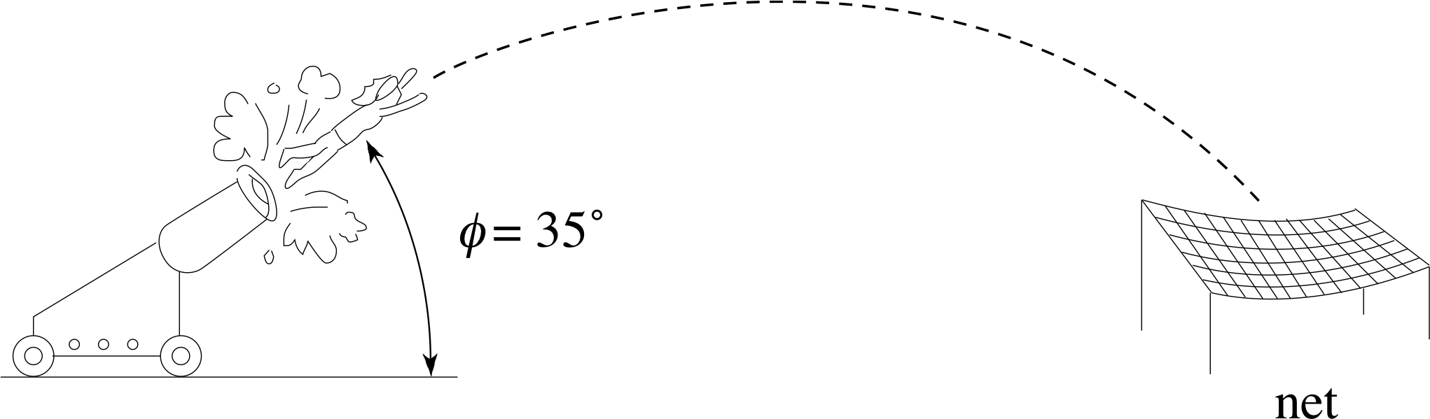
Figure 12 See Answer F1.
Answer F1
Figure 12 illustrates the flight of Miss Magnificent. Her launch speed, υ, is 18 m s−1 and the angle of launch, ϕ is 35°.
If we consider her horizontal motion:
ux = υx = (18 cos 35°) m s−1, the time of flight is T and the range of the flight is R.
If we substitute these (positive) values into
s2 = υxt
we findR = υxT
If we now consider the vertical motion we can find the time of flight T:
Initial vertical velocity, υy = (18 sin 35°) m s−1, on landing sy = 0 m and the time of flight is T.
If we substitute these values into
sy = uyt − ½ gt2(Eqn 20)
we find0 = uyT − ½ gT 2
This equation has two solutions. If we discard the T = 0 solution we obtain:
$T = \dfrac{2u_y}{g} = \rm \dfrac{36\sin35°\,m\,s^{-1}}{9.81\,m\,s^{-2}} = 2.10\,s$
So the range R = υxT = (18 cos 35°) m s−1 × 2.10 s = 31.0 m. Therefore the net must be placed 31.0 m from the launch site.
Question F2
A particle moves in the (x, y) plane from point 1, with position (3 m, 2 m) to point 2, with position (7 m, −1 m).
(a) What are the x– and y–components of the particle’s displacement from point 1 to point 2?
(b) What is the magnitude of this displacement?
(c) What is the angle between this displacement and the x–axis?
Answer F2
(a) Displacement vector from point 1 to point 2:
s = (sx, sy) = (x2− x1, y2− y1) = (4 m, −3 m)
i.e.the x-component of this displacement is 4 m and the y-component is −3 m.
(b) The magnitude of this displacement is given by
$\sqrt{(x_2-x_1)^2+(y_2-y_1)^2} = \rm \sqrt{16+9\os}\,m = 5\,m$
(c) The angle θ is found from the relationship
$\tan\theta = \dfrac{y_2-y_1}{x_2-x_1} = \dfrac{-3}{4} = -0.75$
This gives θ = 323.1° (or −36.9°, where the minus sign implies that the angle is measured in the clockwise sense from the positive x–axis).
Question F3
A shell is fired with a velocity of 200 m s−1 at an angle of 30° above the horizontal. Find the time taken for the shell to reach its maximum height and the magnitude and direction of its velocity after 16 s. Take the magnitude of the acceleration due to gravity to be g = 9.81 m s−2 and ignore the effect of air resistance.
Answer F3
The horizontal (x) and vertical (y) components of the initial velocity are
ux = υy = (200 × cos 30°) m s−1 and uy = (200 × sin 30°) m s−1
Consider the vertical motion first. The maximum height of the vertical motion occurs at υy = 0 m s−2.
Equation 19,
υy = uy − gt(Eqn 19)
gives the time, t, to reach maximum height as
$t = \dfrac{u_y}{g} = \rm \dfrac{(200 \sin 30°)\,m\,s^{-1}}{9.81\,m\,s^{-2}} = 10.2\,s$
To find the vertical component of velocity, υy, after 16 s, we set t = 16 s in Equation 19. This gives us
υy = (20 sin 30°) m s−1 − 9.81 m s−2 × 16 s = −57.0 m s−2
The minus sign indicates that the ball is moving downwards at this time.
Now consider the horizontal motion:
υx = (200 cos 30°) m s−1 = 173 m s−1 (constant)
We can now find the magnitude and direction of the velocity after 16 s. The magnitude υ is found from
$\upsilon = \sqrt{\smash[b]{\upsilon_x^2+\upsilon_y^2}} = \rm \sqrt{\smash[b]{(173)^2 + (-57)^2}}\,m\,s^{-1} = 182\,m\,s^{-1}$
The direction in terms of the angle to the horizontal, ϕ is given by
tan ϕ = υy /υx = (−57.0 m s−1)/173 m s−1 = −0.329
which gives a value for ϕ of −18.2°, i.e. 18.2° below the horizontal.
1.3 Ready to study?
Study comment To begin to study of this module you will need to be familiar with the following terms or topics: Cartesian coordinate system, cosine (as in cos θ), gradientgradient of a line, graph, position coordinates, Pythagoras’s theorem, quadratic equation, SI units, sine (as in sin θ) and tangent (as in tan θ). It is also assumed that you have some familiarity with concepts such as position, speed, velocity and acceleration in the context of one–dimensional linear motion and that you have previously encountered the calculuscalculus notation dx/dt used to indicate the (instantaneous) rate of change of x with respect to t. However, proficiency in the use of calculus is not required for the study of this module. If you are uncertain about any of these items you can review them now by reference to the Glossary, which will also indicate where in FLAP they are developed. The following questions will enable you to check whether you need to review some of the topics before embarking on this module.
Question R1
A right–angled triangle has sides of length a, b and c. If the longest side is of length c and if the angle between that side and side b is θ, write down Pythagoras’s theorem as it applies to this particular triangle and express the lengths a and b in terms of c and θ.
Answer R1
According to Pythagoras’s theorem, a2 + b2 = c2. It follows from basic trigonometry that a = c sin θ and b = c cos θ.
Consult Pythagoras’s theorem and trigonometry in the Glossary for further information.
Question R2
An object moving along the x–axis of a Cartesian coordinate system does so in such a way that its position coordinate x changes from x = −1.0 m to x = 8.0 m in a time interval of 3.0 s. What is the average velocity, $\langle \upsilon_x\rangle$, of the object over the three–second interval? In what way would your answer have been different if the initial and final values of x had been interchanged?
Answer R2
In this sort of one–dimensional motion the average velocity (more properly the average component of velocity in the x–direction) is equal to the rate of change of the position coordinate over the time interval concerned. In this case
$\upsilon_x = \dfrac{x_{\rm final}-x_{\rm initial}}{3\,{\rm s}} = \dfrac{8.0\,m-(-1.0\,m)}{3\,m} = \dfrac{9.0\,m}{3\,s} = 3.0\,m\,s^{-1}$
If the initial and final positions had been interchanged, the sign of the answer would have changed and we would have had υx = −3.0 m s−1. This would have indicated that the object was travelling in the opposite direction, the direction of decreasing x.
Consult average velocity and position coordinate in the Glossary for further information.
Question R3
A cyclist is travelling due north along a straight road at 10 m s−1 when the brakes are applied. If the brakes can cause the speed to reduce at a constant rate of 3 m s−2, how long will it take to stop the bicycle and how far will it have travelled in that time?
Answer R3
The initial velocity, u2 = 10 m s−1; the final velocity, υ2 = 0 m s−2 and the acceleration, a2 = −3 m s−2.
The time, t, taken to stop can be found from one of the uniform acceleration equations for linear motion:
υx = ux + axt
i.e.$t = \dfrac{\upsilon_x-v_x}{a_x} = \dfrac{-10\,m\,s^{-1}}{-3\,m\,s^{-2}} = 3.33\,s$
To find the distance travelled by the bicycle in this time we substitute the known values into another of the uniform acceleration equations for linear motion: υ2 = u2 + 2axsx
so$s_x = \dfrac{\upsilon_x^2-v_x^2}{2a_x} = \rm \dfrac{-100\,m^2\,s^{-2}}{-2\times3\,m\,s^{-2}} = 16.7\,m$
Consult uniform acceleration equations in the Glossary for further information.
2 Describing the motion of a projectile
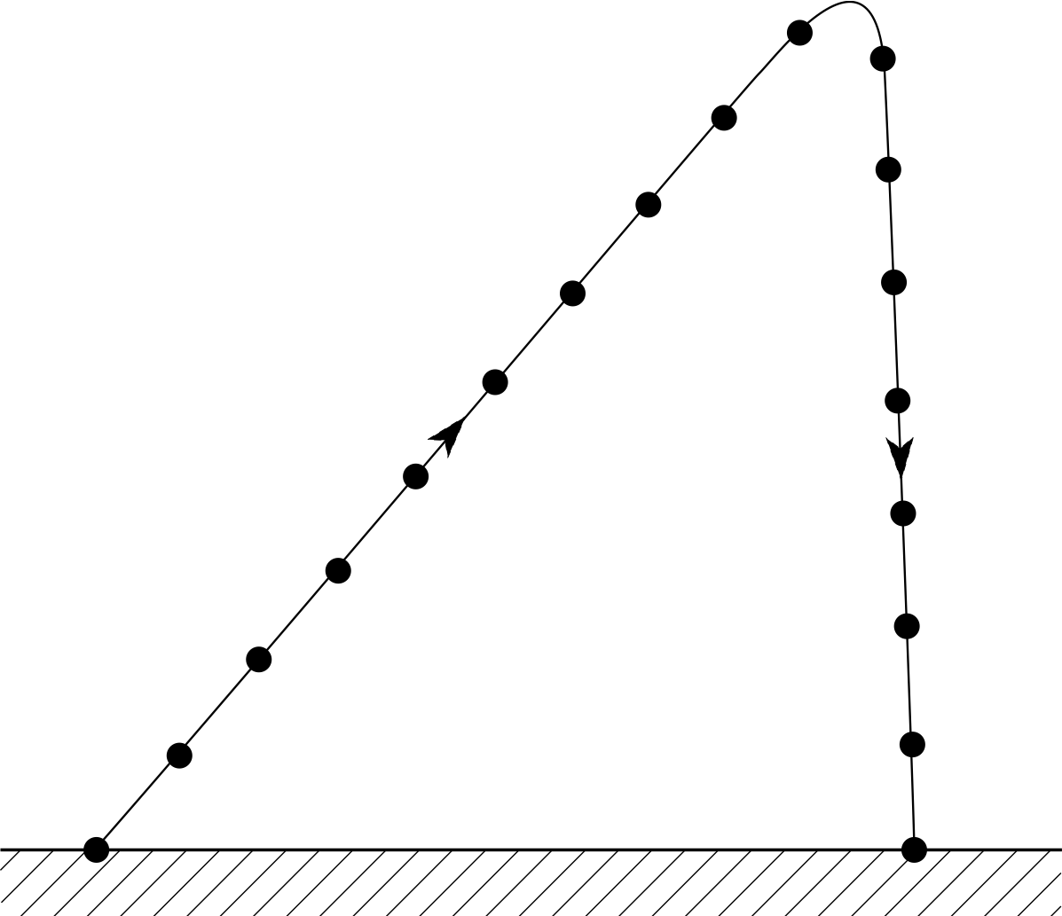
Figure 1 Aristotle’s idea of projectile motion. The dots represent successive positions of the projectile at equally separated moments of time.
Any object that is launched into unpowered flight near the Earth’s surface is called a projectile. A rock thrown from a hand or an arrow released from a bow would be typical examples. The motion of a projectile has been of interest since ancient times, but describing the motion accurately and explaining its cause has created a great deal of difficulty. In the 4th century BC the Greek philosopher Aristotle (384–322 BC) said that when an object is thrown it will carry on in a straight line until it runs out of ‘force’, after which it will fall down. Figure 1 illustrates his idea, which we will soon see to be incorrect.
In medieval times the exact paths of cannonballs and arrows were of great interest, and it became necessary to think about them more precisely.
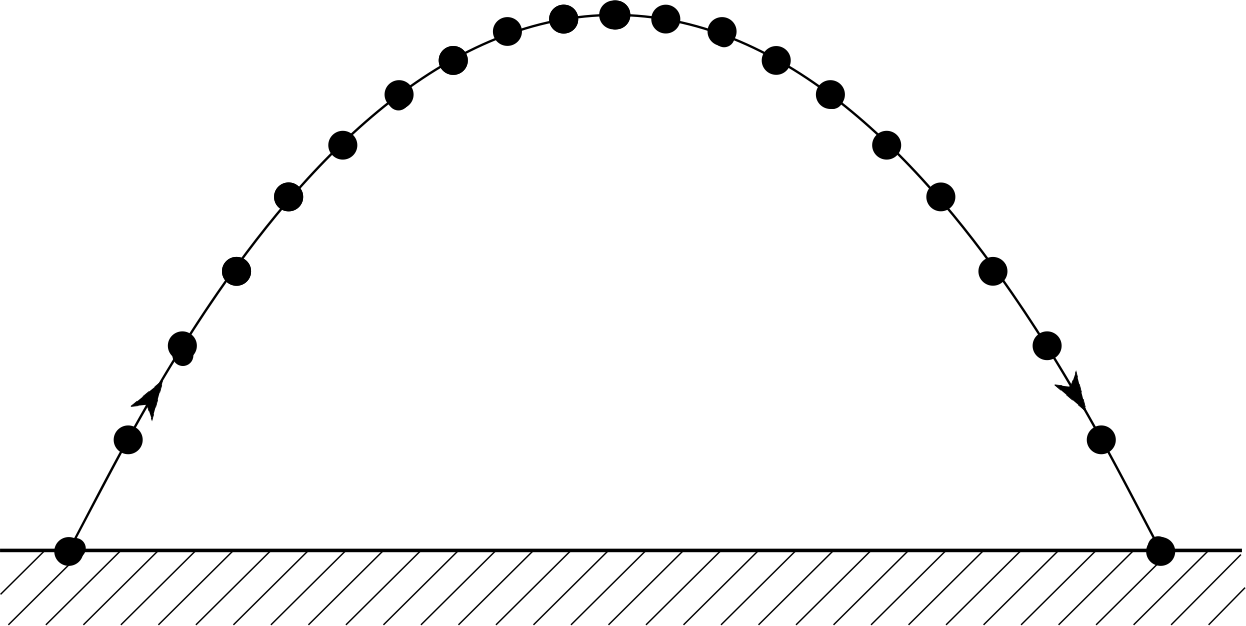
Figure 2 Galileo’s idea of projectile motion. Note how the dots representing successive positions of the projectile bunch together near the top of the trajectory.
In the 16th century the Italian scientist Galileo Galilei (1564–1642) produced an accurate analysis of the flight path, or trajectory, of a projectile, this is illustrated schematically in Figure 2.
In this module we will be concerned only with projectiles that may be treated as particles (i.e. bodies with negligible size and no internal structure, that may be regarded as occupying a single point in space at any particular time). Also we will assume that during flight, projectiles move under the influence of gravity alone; in other words we will ignore air resistance and other such effects. These restrictions may seem rather limiting, but for many purposes the motion of quite large bodies, such as footballs and people, can often be modelled quite successfully on this basis.
Of course, there are many problems in which these simplifications would be misleading. Real projectiles have a finite size and this allows air resistance to influence their motion. When air resistance is large it cannot be ignored, for example, badminton players will recognize the trajectory of a shuttlecock as being nearer to that shown in Figure 1 than Figure 2. Also, in many ball games, such as cricket and tennis, it is possible to spin the ball. The effect of this spin on the flow of air around the ball produces a sideways force so that the ball ‘swerves’. These phenomena are beyond the scope of this module, though it is not too difficult to extend the ideas that are introduced here in order to accommodate them.
2.1 Position and displacement
Study comment This subsection is mainly concerned with vector notation and deliberately parallels the development of vectors presented in the maths strand of FLAP. If you have already studied vectors there or elsewhere you should aim to finish this subsection very quickly, pausing only to make sure that you are familiar with the notation that will be used in this module and that you are able to answer Questions T1 and T2. If you are unfamiliar with vectors and you feel you need a more detailed treatment than that presented here you should consult the Glossary which will refer you to the appropriate modules in the maths strand.
Position
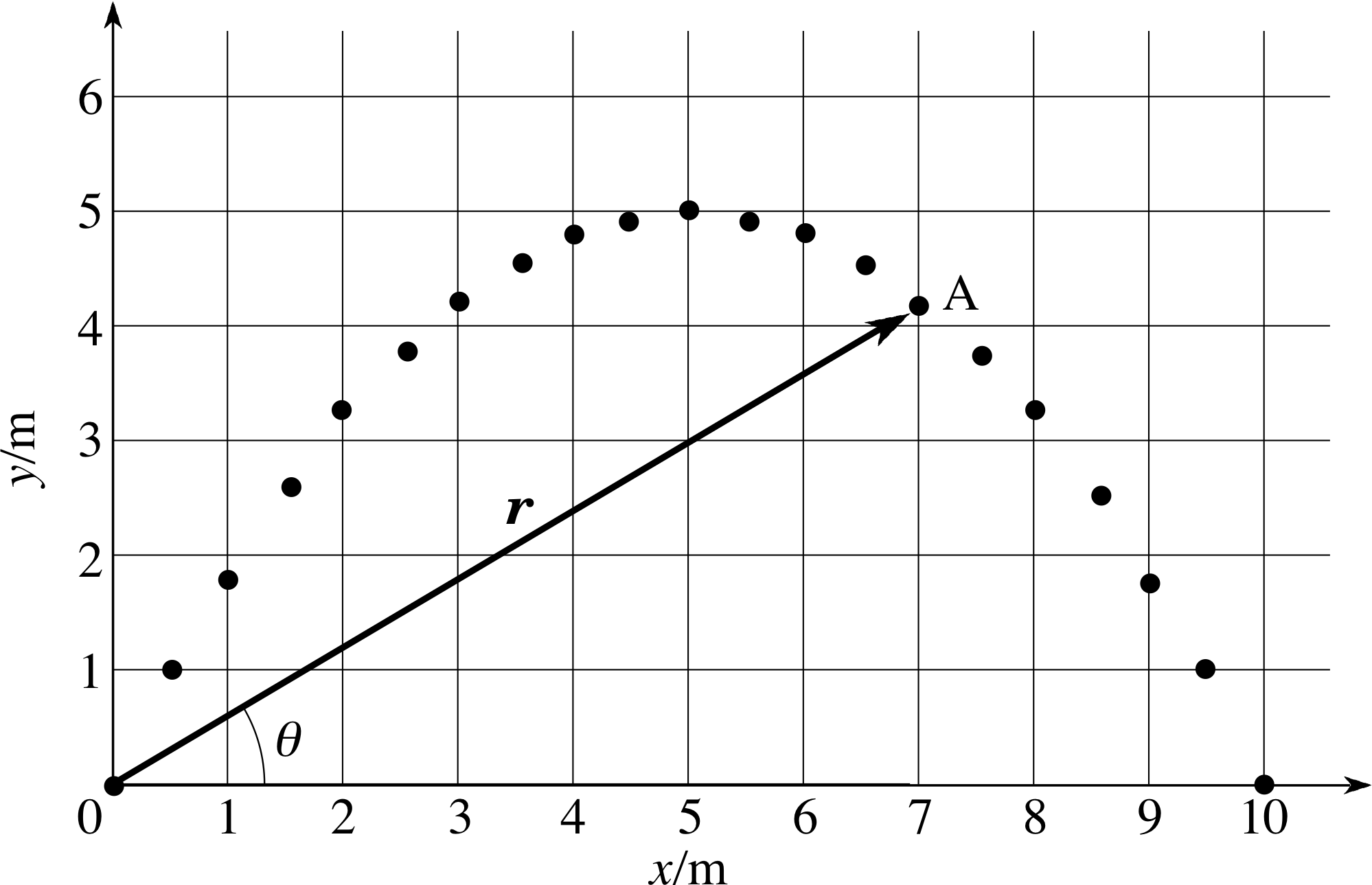
Figure 3 The arrow drawn from the origin to a point such as A represents the position vector r of that point.
A projectile represented by a point particle moving under the influence of gravity has a trajectory that is confined to a single vertical plane. Such a projectile is said to exhibit two–dimensional motion, since its trajectory may be adequately described using just two independent coordinate axes. In this module we will use two mutually–perpendicular Cartesian coordinate axes for this purpose: a horizontal axis which will usually be labelled x, and a vertical axis which will usually be labelled y. These axes meet at a point called the origin from which we can measure the position coordinates of any point in the plane of the axes (i.e. the specific values of x and y that determine the location of that point in the plane). So, provided we choose the directions of the x- and y–axes appropriately, we can suppose that the motion of any projectile we wish to consider is confined to the (x, y) plane and may be described in terms of the changing values of the projectile’s x- and y–coordinates.
Figure 3 uses a two–dimensional Cartesian coordinate system of the sort just described to show various points along the trajectory of a projectile launched from the origin (the point marked O). As usual, the dots represent successive positions of the projectile at equally separated moments of time. The location of any point on the trajectory, such as the point marked A, can be described in terms of its position coordinates. In this particular case we can call them xA and yA since they relate to the point A, and we can adopt the convention of writing them as an ordered pair, (xA, yA), in which the first value is always the x–coordinate and the second the y–coordinate.
✦ What are the position coordinates (xA, yA) of point A in Figure 3?
✧ Point A is located at x = 7.0 m and y = 4.2 m, so (xA, yA) = (7.0 m, 4.2 m)
Figure 3 The arrow drawn from the origin to a point such as A represents the position vector r of that point.
Figure 3 also indicates an alternative way of specifying the location of a point in the (x, y) plane. An arrow of given length and given orientation, with its tail at the origin, will inevitably have its tip at some specific point. Such an arrow is called the position vector of the point and is generally denoted by the bold symbol r. The bold symbol is used to distinguish the position vector (which has both magnitude and direction) from its magnitude r which is the distance of the point from the origin of coordinates. A distance r doesn’t point in any particular direction and does not specify a point; a position vector r has direction and does specify a point.
Note that in order to specify the position vector r of a particular point we must clearly define two things:
- 1
-
the magnitude_of_a_vector_or_vector_quantitymagnitude of r, which is the distance r from the origin to the point in question;
- 2
-
the direction_of_a_vectordirection of r, which in two dimensions can be described by the angle θ measured in an anticlockwise direction from the positive x–axis to r.
✦ Using a ruler and a protractor determine the magnitude and direction of the position vector r of point A. i
✧ Working to two significant figures, the magnitude of r is r = 8.2 m, and its direction in the plane is given by the angle θ = 31°.
Aside As has already been stressed, position vectors and their magnitudes may both be represented by the same letter, but the vector is distinguished by the use of a bold typeface. This is fine in print but not of much help in work that you have to write by hand. In order to show that a handwritten letter is supposed to represent a vector you should generally put a wavy underline beneath it as in $\underset{\sim}{\it a}$. This sort of underline is used to indicate to a printer that whatever has been underlined should be set in bold type.
So, we now have two different ways of specifying the location of any point in the (x, y) plane. We can either give the coordinates of the point (x, y) or we can specify the point’s position vector r by giving its magnitude and direction. There is clearly an intimate relationship between these two descriptions. Indeed, it is natural to use the ordered pair of position coordinates (x, y) as a way of identifying the position vector r by writing
r = (x, y)(1)
When represented in this way we say that x and y are the components_of_a_vectorcomponents of the position vector r. Thus, we may say that the point A in Figure 3 has the position vector r = (7.0 m, 4.2 m) or, equivalently, we may say that the x–component of r is 7.0 m, and that the y–component of r is 4.2 m.
For a two–dimensional position vector, the magnitude r is related to the components x and y by Pythagoras’s theorem:
$r = \sqrt{x^2+y^2}$(2)
where $\sqrt{x^2+y^2}$ indicates the positive square root of x2 + y2. Note that this relation ensures that the magnitude of the position vector will be a positive quantity as any length must be. It is often useful to emphasize this by using the symbol | r | to represent the magnitude of r. You might forget that r represents a positive quantity, but you are unlikely to forget that | r | must be positive.
The direction of a position vector may also be related to its components. For the two–dimensional position vector r = (x, y), the direction of which is specified by the angle θ, the relationship takes the form
$\tan\theta = \dfrac{x}{y}$(3) i
It also follows from basic trigonometry that the horizontal and vertical components of a position vector r are
x = r cos θ and y = r sin θ(4)
sor = (r cos θ, r sin θ)(5)
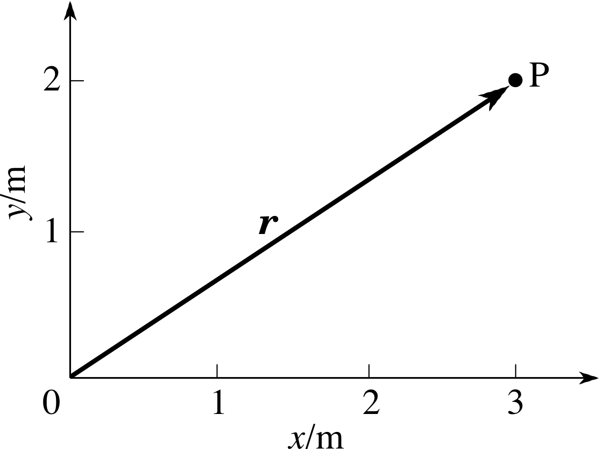
Figure 4 A point P with its position vector, r.
Question T1
Figure 4 shows a point P and its position vector r. Write down the position coordinates of the point, P, and use those coordinates to determine the magnitude and direction of the position vector r.
Answer T1
r = (3 m, 2 m)
$\lvert\,\boldsymbol r\,\rvert = \rm \sqrt{13\os}\,m = 3.6\,m$
tan θ = y/x = 2/3
andθ = 33.7° where θ is the angle with the +x–axis.
Position vectors are not the only quantities with magnitude and direction that are of interest to us in the study of projectile motion, or indeed in physics generally. In fact, any quantity that requires both a magnitude and a direction for its complete specification is called a vector, and common examples that you will meet in this module include velocity and acceleration. As you will see later, any vector may be expressed in terms of its components though in most cases the components will not have such a simple interpretation as the components of a position vector.
Many physical quantities, such as mass, length, time, speed and temperature, are specified by a magnitude alone. Such quantities are collectively called scalars. Although scalars are quite distinct from vectors it should be noted that the components of a vector are actually scalar quantities (they are sometimes formally referred to as scalar components for this reason).
Thus, although it would not make sense to equate a vector (which involves direction) with a scalar (which does not), it is possible to identify a vector with an ordered arrangement of scalars such as (7.0 m, 4.2 m) since it is the agreed ordering and the predefined coordinate system that supplies the directional information.
A vector is a quantity that is characterized by a magnitude and a direction. By convention, bold typeface symbols such as r are used to represent vector quantities. The magnitude of such a vector is represented by | r | or r and is a non–negative scalar quantity. In diagrams, vectors are represented by arrows or directed line segments. In handwritten work vectors are distinguished by a wavy underline ($\,\underset{\sim}{\it a}\,$) and the magnitude of a vector is denoted $\lvert\,\underset{\sim}{\it a}\,\rvert$.
Displacement
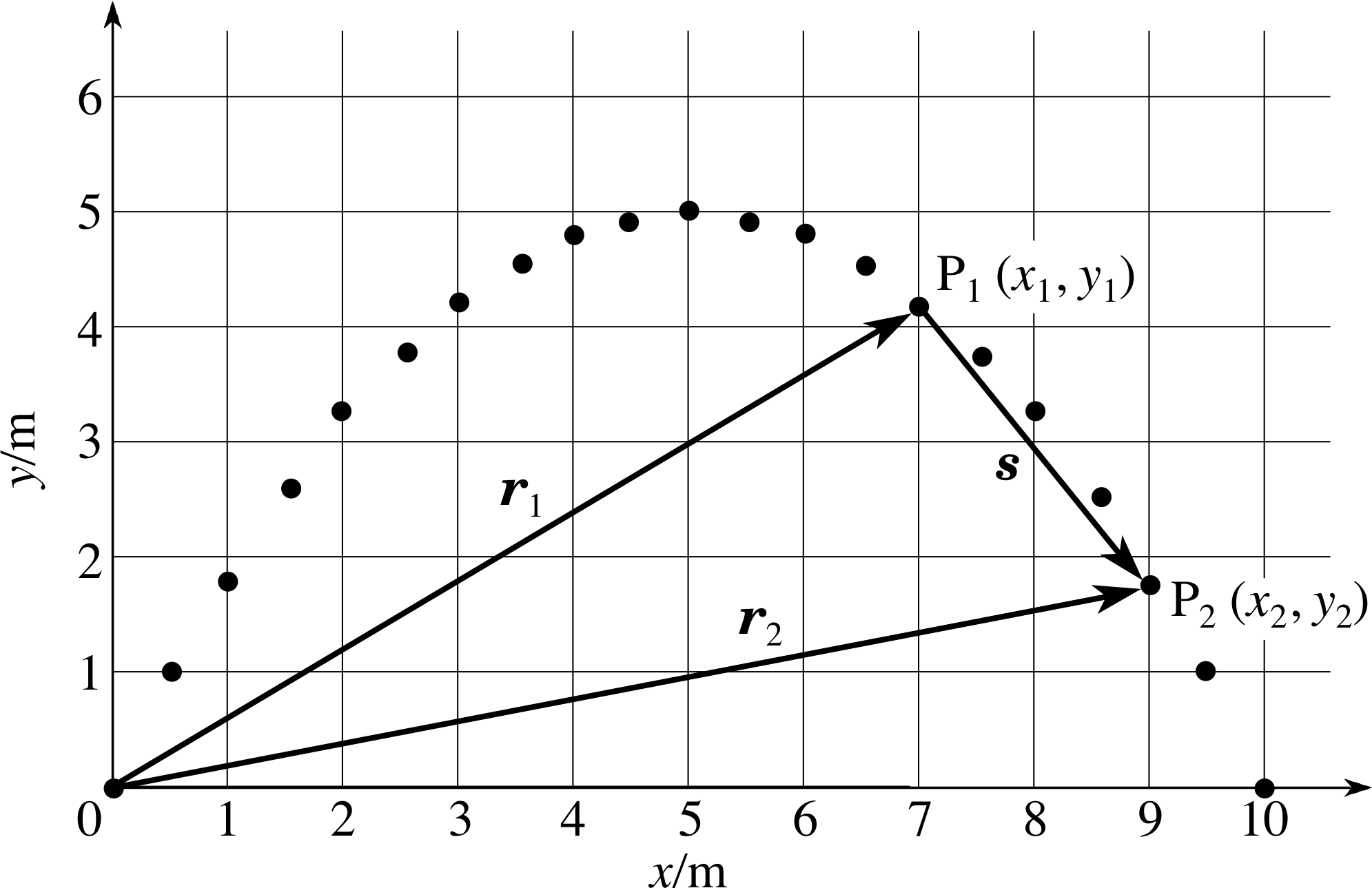
Figure 5 Displacement and position vectors.
In many projectile problems a vector quantity that is of particular interest is displacement which can be used to describe a change or a difference in position. The distinction between the position and displacement vectors can be seen from Figure 5 in which O is the origin of a Cartesian coordinate system from which the changing position of a projectile can be measured. During part of its motion the projectile moves from P1 (with position vector r1 = (x1, y1)) to P2 (with position vector r2 = (x2, y2)). The corresponding change (or difference) in the projectile’s position can be represented by the arrow marked s in Figure 5. This is certainly a vector quantity since it has both magnitude and direction, but it cannot be a position vector because its tail is not at the origin. It is in fact the displacement from P1 to P2.
Like all vectors, the displacement s from P1 to P2 can be expressed in terms of its components. These are generally denoted by sx and sy; so we can write s = (sx, sy), where sx and sy, respectively, represent the differences in the x– and y–coordinates of P1 and P2:
sx = (x–coordinate of P2) − (x–coordinate of P1) = x2 − x1
sy = (y–coordinate of P2) − (y–coordinate of P1) = y2 − y1
Thus,s = (sx, sy) = (x2 − x1, y2 − y1)(6)
✦ What are the components of the particular displacement shown in Figure 5? Use your answers to write the vector as an ordered pair of components.
✧ sx = 9.0 m − 7.0 m = 2.0 m, sy = 1.8 m − 4.2 m = −2.4 m.
Hence, s = (2.0 m, −2.4 m).
The great advantage of using displacements rather than position vectors when describing projectile motion is that the displacement from one point to another does not depend in any way on where the origin of the coordinate system is located. For instance, even if we moved the origin of coordinates in Figure 5 from the origin to some other point, it would still remain true that the displacement from P1 to P2 is s = (2.0 m, −2.4 m); choosing a new origin would change the position coordinates and position vectors of P1 and P2, but it would not change the differences that determine sx and sy. i Why is this an advantage? In projectile problems we are usually interested in how far the projectile has travelled (horizontally or vertically) from its launch point. If we describe the motion in terms of displacements from the launch point rather than positions relative to the origin we will have a description (in terms of displacements) that will be equally valid whether or not the launch point happens to be at the origin. In Figure 5 the launch point was at the origin, but that won’t always be the case.
Although we have gone to some lengths to stress the differences between position vectors and displacements it is important to realize there are also deep similarities. A displacement vector provides us with a way of describing the location of one point (such as P2) with respect to some arbitrarily chosen reference point (such as P1). A position vector provides us with a way of describing the location of one point (such as P2) with respect to a very particular reference point – the origin O. Clearly, if we were to choose O as the arbitrary reference point from which we measured displacements then the displacement of a point such as P2 would be equal to its position vector. To this extent position vectors are simply a special class of displacements; position vectors are displacements from the origin.
2.2 Vector algebra
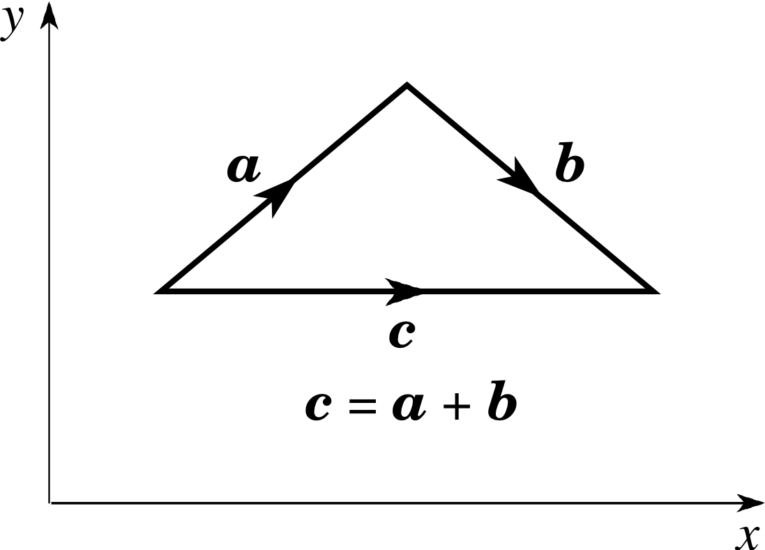
Figure 6 The triangle rule for adding vectors. Note the directions of the arrows: the diagram would be incorrect if any one, or any two of the arrows were reversed.
It is a general property of displacements that they can be added together, though the word ‘added’ has to be interpreted in a rather special way. For example, the projectile launched from point O in Figure 5 will at some stage arrive at point P1, where its displacement from O is r1, i and some time later, after undergoing a further displacement s from P1, it will arrive at P2 where its displacement from O is r2. Consequently it makes sense to say that the result of adding the displacement s to the displacement r1, is the displacement r2. More formally we say that r2 is the vector sum or resultant_vectorresultant of r1 and s and we write
r2 = r1 + s
The operation of adding vectors together is called vector addition, the process is not restricted to displacements but it can only be applied to vectors of ‘similar type’, e.g. we can add a velocity to a velocity, or an acceleration to an acceleration, but we cannot add a velocity to an acceleration.
A vector sum such as r1 + s looks a lot like an ordinary (scalar) sum, but it is really quite different because the directions of the vectors must be taken into account as well as their magnitudes. When thinking about vector addition you should have in mind a picture something like that shown in Figure 6, the essential features of which are described by the following rule:
The triangle rule for adding vectors:
Let a and b be vectors of similar type represented by appropriate arrows (or directed line segments). If the arrow representing b is drawn from the head of the arrow representing a, then an arrow from the tail of a to the head of b represents the vector sum c = a + b.
✦ If c = a + b, will it necessarily be the case that | c | = | a | + | b |?
✧ No, looking at Figure 6 you can see that the magnitude of c (i.e. its length) is less than the sum of the magnitudes of a and b.
Although it is helpful to have a picture in mind when thinking about vector addition, it is usually easier to perform such additions with the aid of components. For instance, looking at Figure 6 you should be able to a convince yourself that if a = (ax, ay), b = (bx, by) and c = (cx, cy) then the vector equation a + b = c may be written in the form
(ax, ay) + (bx, by) = (cx, cy)
where cx = ax + bx
andcy = ay + by
In other words,
To add together vectors a and b, simply add the corresponding components so that:
a + b = (ax, ay) + (bx, by) = (ax + bx, ay + by)(7)
✦ If c = a + b, where a = (1.6 m, −5.5 m) and b = (−1.6 m, 5.3 m), express c in terms of its components and describe its direction in words.
✧ c = (0 m, −0.2 m). If the y–axis points vertically upwards, the vector c points vertically downwards.
Apart from adding vectors another useful mathematical operation that can be carried out is that of multiplying a vector by a scalar. This is called scaling_of_a_vectorscaling and may be defined in the following way
To multiply a vector a by a scalar λ, simply multiply each component of a by λ so that:
λa = λ (ax, ay) = (λax, λay)(8)
The result of scaling a by λ is to produce a vector λa of magnitude | λa | = | λ | | a | that points in the same direction as a if λ is positive, and in the opposite direction to a if λ is negative. So, for example, given a displacement a, the scaled vector 2a would be twice as long and would point in the same direction, and the scaled vector −a = (−1)a would have the same length as a but would point in the opposite direction (i.e. it would be antiparallel) to a.
✦ If a = (−7 m, 4 m) and b = (−1 m, 2 m) what are the components of the vector a − 4b? What is the magnitude of a − 4b?
✧ a − 4b = (−7 m, 4 m) + (4 m, −8 m) = (−3 m, −4 m)
$\lvert\,\boldsymbol{a}- 4\boldsymbol{b}\,\rvert = \rm \sqrt{(-3\,m)^2 +(-4\,m)^2} = 5\,m$
Figure 5 Displacement and position vectors.
Now that you know how to add and scale vectors you should be able to rearrange vector equations. For instance, referring back to Figure 5 and recalling that r1 = (x1, y1), r2 = (x2, y2) and s = (x2 − x1, y2 − y1), it is easy to see that the vector equation r2 = r1 + s can be rearranged to give a purely vectorial definition of displacement:
s = r2− r1
Given the rule for adding vectors, it should be pretty clear what we mean by a vector difference such as r2 − r1 but if you are in any doubt just regard the vector difference as the sum of r2 and the scaled vector (−1)r1. It then follows from the above definitions that
s = r2 − r1 = (x2, y2) − (x1, y1) = (x2 − x1, y2 − y1)(9)
As you can see, vector equations can be treated very much like ordinary equations as far as rearrangements are concerned, though you should keep in mind the directional nature of vectors so that you avoid trying to do something silly like dividing by a vector.
Another possible rearrangement of r2 = r1 + s is
r2 − r1 − s = 0
where 0 = (0, 0) represents the zero vector which has zero magnitude. (Note that a vector cannot be equal to a scalar, so you should always write a − a = 0 rather than a − a = 0).
Question T2
A body moves from a point A, with position coordinates (4 m, 2 m), to a point B, with position coordinates (7 m, −3 m). What is the magnitude and direction of this displacement? Check your answers by drawing a scale diagram.
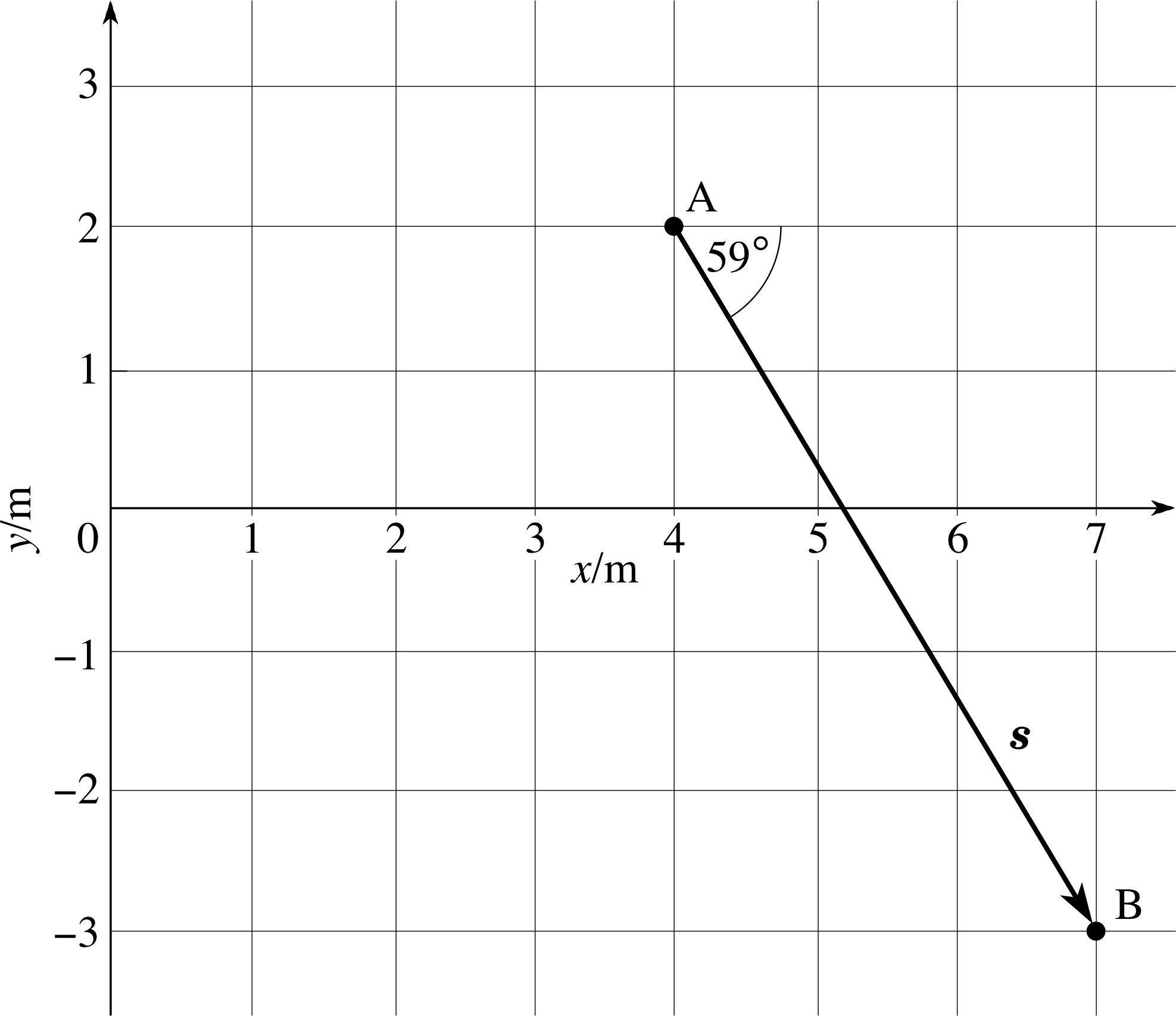
Figure 13 See Question T2.
Answer T2
The displacement s = (sx, sy) = (x2− x1, y2− y1)
s = (3 m, −5 m)
i.e.sx = 3 m and sy = −5 m
The magnitude of this displacement
$s = \sqrt{(x_2-x_1)^2+(y_2-y_1)^2}$
so$s = \rm \sqrt{3^2+(-5)^2}\,m = 5.83\,m$
The direction of this displacement is given by
$\tan\theta = \dfrac{(y_2-y_1)}{(x_2-x_1)} = \dfrac{-5}{3}$
which gives θ = 301.0° (i.e. −59.0°)
Figure 13 is a scale drawing of this displacement. The measured values of sx, sy, θ and the magnitude of the displacement agree with those calculated.
2.3 Velocity in projectile motion
Let us return yet again to the kind of projectile motion shown in Figure 5, but let us now associate values of the time with various points in the motion. In particular suppose that at time t the projectile passes through a point P with position vector r = (x, y), and that a short time later, at t + ∆t, the projectile arrives at a point with position coordinates (x + ∆x, y + ∆y). i We can then represent the change in position over the short time ∆t by the displacement vector ∆r = (∆x, ∆y) and we can define the average velocity $\langle\upsilon\rangle$ of the projectile as it moves between the two points by
$\langle\upsilon\rangle = \dfrac{\Delta \boldsymbol{r}}{\Delta t}=\dfrac{1}{\Delta t}(\Delta x,\,\Delta y) = \left(\dfrac{\Delta x}{\Delta t},\,\dfrac{\Delta x}{\Delta t}\right)$(10) i
Note that the operation of dividing the two–dimensional displacement ∆r by ∆t really amounts to scaling ∆r by 1/∆t, so the resulting average velocity is another two–dimensional vector that points in the same direction as ∆r. The x–component of $\langle\upsilon\rangle$ is given by ∆x/∆t and represents the average rate of change of the x–coordinate of the projectile, while the y–component, ∆y/∆t, represents the average rate of change of the projectile’s y–coordinate. This definition of the average velocity vector provides the natural two–dimensional generalization of the definition given elsewhere in FLAP for average velocity in one–dimensional (linear) motion. In effect the two–dimensional velocity can be regarded as the result of two independent linear velocities, one in the x–direction and the other in the y–direction.
In practice we often need to know the velocity of a projectile at a particular instant, rather than the average velocity over some specified interval. This instantaneous velocity υ is also a vector quantity, the components of which, υx and υy, can be found by considering the corresponding components of average velocities taken over smaller and smaller intervals around the time in question. In mathematical terms we can indicate that the instantaneous velocity is a limiting case of the average velocity as the time interval ∆t becomes vanishingly small by writing
$\displaystyle \langle\upsilon\rangle = \lim_{\Delta t\rightarrow 0}\dfrac{\Delta \boldsymbol{r}}{\Delta t} = \lim_{\Delta t\rightarrow 0}\dfrac{1}{\Delta t}(\Delta x,\,\Delta y) = \left[\lim_{\Delta t\rightarrow 0}\left(\dfrac{\Delta x}{\Delta t}\right),\,\lim_{\Delta t\rightarrow 0}\left(\dfrac{\Delta x}{\Delta t}\right)\right]$(11)
Now, if you are familiar with calculus you will know that limits of this kind are represented symbolically by derivatives, so we have
${\boldsymbol\upsilon} = \dfrac{d{\boldsymbol{r}}}{dt} = \left(\dfrac{dx}{dt},\,\dfrac{dy}{dt}\right)$(12)
and since we can write υ = (υx, υy) we can see that
$\upsilon_x = \dfrac{dx}{dt} \quad\text{and}\quad\upsilon_y = \dfrac{dy}{dt}$
Whether you are familiar with calculus or not i, you should be able to appreciate that these final equations have a simple graphical interpretation. If you were to draw a graph showing how the x–coordinate of the projectile changed with time (i.e. an x against t graph) then the gradient (i.e. slope) of that graph at any particular value of t would represent the instantaneous velocity component υx at that time. Similarly, the gradient of a y against t graph at any particular value of t would represent the value of υy at that time. Thus, each component of the projectile’s instantaneous velocity represents the instantaneous rate of change of the corresponding component of the projectile’s position vector.
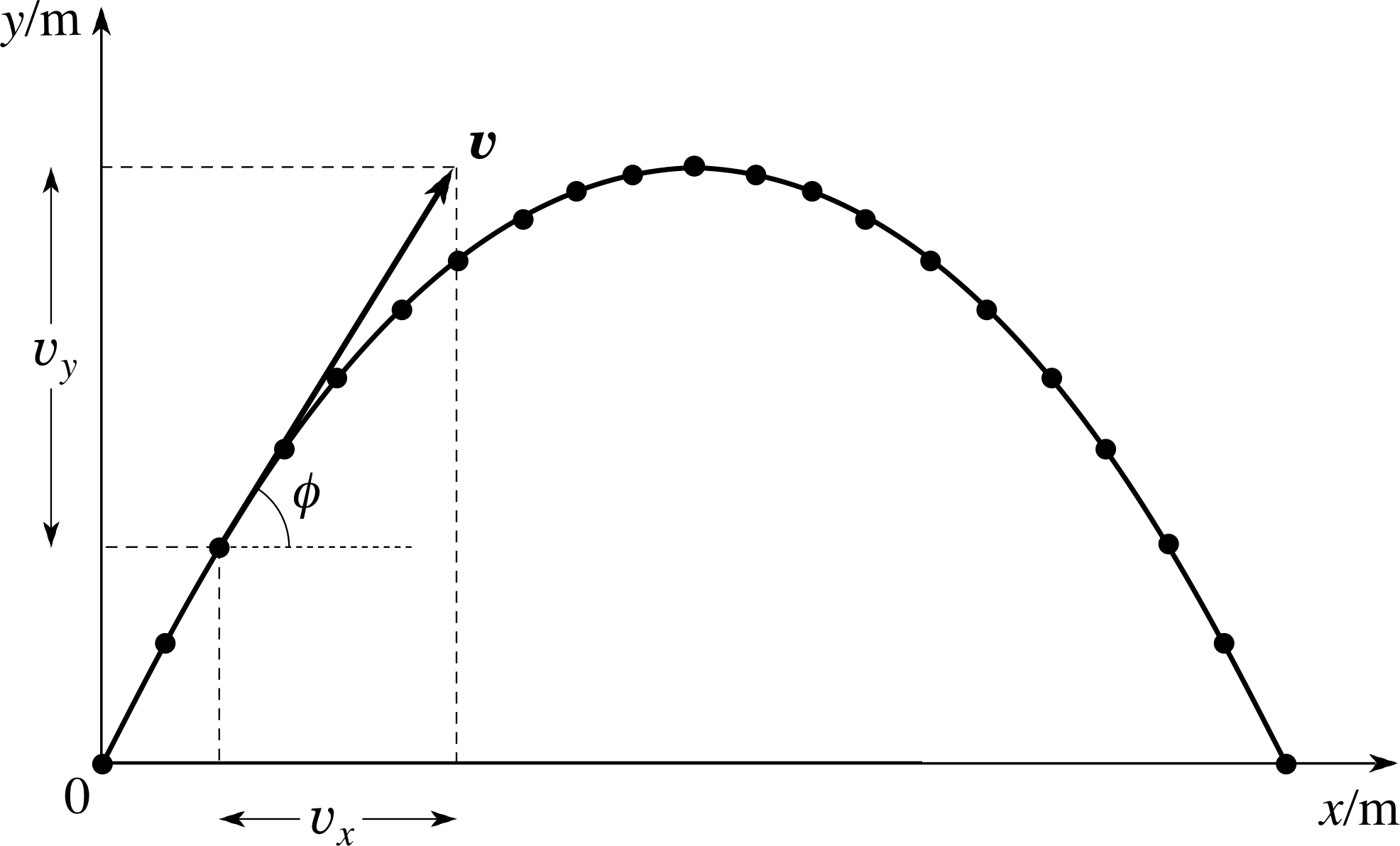
Figure 7 The instantaneous velocity v = (vx, vy) of a projectile is tangential to the trajectory at any point.
It follows that the instantaneous velocity itself is the instantaneous rate of change of the position vector and at any particular time it is tangential to the trajectory (see Figure 7).
In discussing the velocity i of a projectile we have, so far, emphasized the use of components but, as you know, a vector can also be characterized by its magnitude and direction. The magnitude of the (instantaneous) velocity υ is called the (instantaneous) speed and may be represented by υ or | υ |: it is of course a scalar quantity and it can never be negative. Thus, it makes perfectly good sense to say that the velocity component υy = −2.4 m s−1, but it would be utter nonsense to say that the speed υ had the same value. For the two–dimensional motion of a projectile, the direction of the velocity υ can be described by the angle ϕ (measured in the anticlockwise direction) between the positive x–axis and the velocity vector (see Figure 7).
So, given a velocity υ we can write down the following relationships
υ = (υx, υy)
withυ = | υ | = $\sqrt{\smash[b]{\upsilon_x^2+\upsilon_y^2}}\quad\text{and}\quad\tan\phi = \dfrac{\upsilon_y}{\upsilon_x}$
orυx = υ cos ϕ and υy = υ sin ϕ
Study comment Notice that in Figure 7 we have used ϕ to represent the angle between υ and the x–axis, whereas in Figure 3 we used θ to represent the angle between r and the x–axis. In problems involving projectile motion we must be careful never to confuse these two angles, which are usually quite different. In this module we will reinforce the distinction by always using the appropriate symbol for each angle.
Question T3
Find the magnitude and direction of a velocity which has an x–component υx, of 8 m s−1 and which has a y–component υy, of 10 m s−1.
Answer T3
The magnitude of the velocity, υ is given by
$\upsilon = \sqrt{\smash[b]{(\upsilon_x^2+\upsilon_y^2)}} = \rm \sqrt{8^2+10^2}\,m\,s^{-1} = 12.8\,m\,s^{-1}$
The direction is given by the angle to the horizontal, ϕ where
$\tan\phi = \dfrac{\upsilon_y}{\upsilon_x} = \dfrac{10}{8} = 1.25$
which gives ϕ = 51.3°
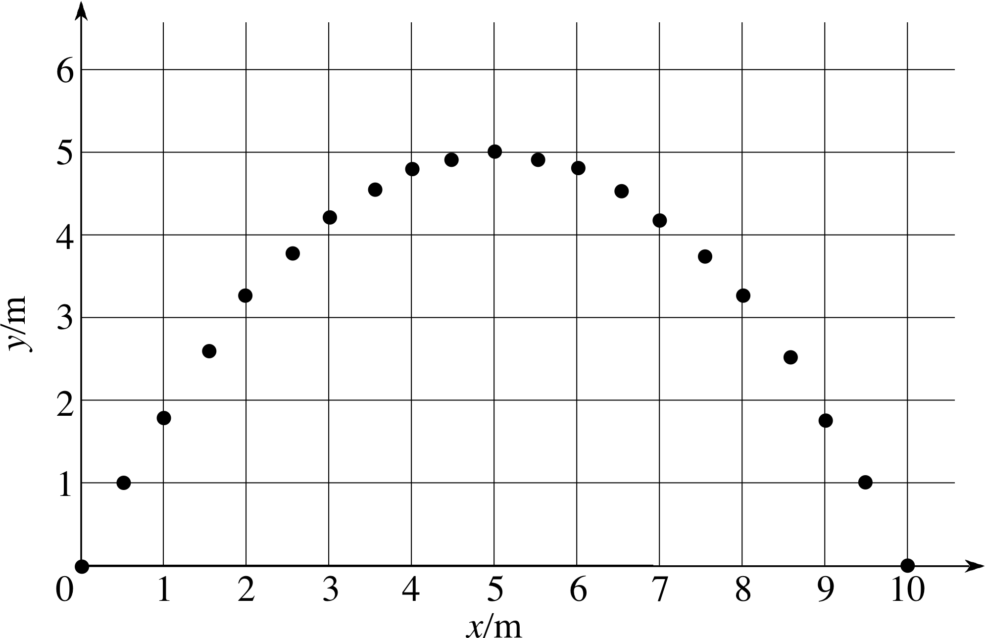
Figure 8 Successive positions of a projectile at intervals of 0.1 s.
Figure 8 is an enlarged version of Figure 3, without the position vector. We can use this diagram to investigate the motion of the projectile in the x– and y–directions. The dots represent successive positions of the projectile at intervals of 0.1 s.
Question T4
Using Figure 8, measure the x–component of the displacement between the first and second, second and third, eighth and ninth, fourteenth and fifteenth, and sixteenth and seventeenth dots. What do your answers suggest about the x–component of the projectile’s velocity?
Answer T4
The x–displacements are all 0.5 m. Therefore the ball undergoes equal displacements in the horizontal direction in equal time intervals. This implies that the x–component of the velocity, υx, is constant.
It seems from the solution to Question T4 that the horizontal component of the velocity of a projectile is constant.
We can also use Figure 8 to try to acquire information about the vertical component of the velocity of a projectile.
Question T5
Using Figure 8, measure the y–component of displacement between the same points as in Question T4. What do these values suggest about the y–component of the projectile’s velocity?
Answer T5
The y–displacement between the first and second dot is 1 m, between the second and third dot it is 0.8 m, between the eighth and ninth it is 0.3m, between the fourteenth and fifteenth −0.4 m, and between the sixteenth and seventeenth dot it is −0.5 m. The displacements in successive time intervals of 0.1 s continuously decrease. Therefore the vertical velocity component is initially positive, decreases as it rises and then becomes increasingly negative as it falls.
From the solution to Question T5, the vertical component of the velocity υy, is not constant. Its value is positive at the launch point but decreases as the projectile ascends, υy = 0 momentarily when the projectile reaches its maximum altitude and thereafter υy is negative and decreasing until the projectile hits the ground. Clearly, if we want to describe the velocity of the projectile more precisely we need some way of describing the rate of change of this vertical component of velocity; that is the function of the next subsection.
2.4 Acceleration in projectile motion
Just as we can use a two–dimensional velocity to describe the rate of change of position of the projectile so we can use a two–dimensional instantaneous acceleration to describe the rate of change of the projectile’s velocity. So, if the velocity of the projectile changes from υ at time t, to υ + ∆υ at time t + ∆t, we can say that the instantaneous acceleration at time t is
$\displaystyle {\boldsymbol a} = \lim_{\Delta t\rightarrow 0}\dfrac{\Delta{\boldsymbol\upsilon}}{\Delta t} = \lim_{\Delta t\rightarrow 0}\left(\dfrac{\Delta{\upsilon_x}}{\Delta t},\,\dfrac{\Delta{\upsilon_y}}{\Delta t}\right) = \left[\lim_{\Delta t\rightarrow 0}\left(\dfrac{\Delta{\upsilon_x}}{\Delta t}\right),\,\lim_{\Delta t\rightarrow 0}\left(\dfrac{\Delta{\upsilon_y}}{\Delta t}\right)\right]$
or, in terms of derivatives
${\boldsymbol a} = \dfrac{d\boldsymbol \upsilon}{dt} = \left(\dfrac{d\upsilon_x}{dt},\,\dfrac{d\upsilon}{dt}\right)$(13)
In terms of components,
a = (ax, ay)
where$a_x = \dfrac{d\upsilon_x}{dt} \quad\text{and}\quad a_y = \dfrac{d\upsilon_y}{dt}$
As usual we can interpret these equations graphically: the value of ax at any particular time is given by the gradient of the υx against t graph at that particular time, and similarly for υy.
✦ Express the magnitude of the instantaneous acceleration a in terms of its components ax and ay, and then express the components in terms of the magnitude and the angle ψ i from the positive x–axis to a.
✧ $a = \lvert\,\boldsymbol{a}\,\rvert = \sqrt{\smash[b]{a_x^2 + a_y^2}}$
The components are: ax = a cos ψ and ay = asin ψ
In what follows we will generally refer to the instantaneous acceleration simply as the acceleration. You learned in the last subsection that one characteristic of projectile motion is that the horizontal component of velocity υx, is constant. This means that the rate of change of υx must be zero and consequently ax = 0.
You also learned that the vertical component of the velocity changes continuously throughout the motion. Careful measurements would show that in the absence of air resistance υy decreases at a constant rate. In other words, throughout the motion the vertical component of velocity is reduced by equal amounts ∆υx in equal intervals of time ∆t, irrespective of when those intervals begin and end. It follows that the vertical component of acceleration is a negative constant which we can write as ay = −g. Since this vertical component of acceleration is caused by the action of gravity on the projectile we say that the constant g is the magnitude of the acceleration due to gravity.
The value of g varies from place to place over the Earth’s surface, but it is generally about 9.8 m s−2 and is usually taken to be 9.81 m s−2 throughout the UK. It describes the acceleration with which all objects near the surface of the Earth fall, so long as they are not impeded appreciably by air resistance.
Combining the observations that ax = 0 and ay = −g we have:
a = (ax, ay) = (0, −g)(14)
and a = | a | = g It is this particular acceleration that characterizes a projectile near the Earth’s surface (in the absence of air resistance).
✦ If you were to measure the speed of a projectile at two different times separated by an interval of one second would you always expect them to differ by about 9.8 m s−1? If not, under what conditions would you expect the speeds to differ by about 9.8 m s−1. (As usual, ignore air resistance, but think carefully!)
✧ No, υy will change by about 9.8 m s−1, but the speed of the projectile is given by an expression of the form $\upsilon = \sqrt{\smash[b]{\upsilon_x^2+\upsilon_y^2}}$ where υx is a constant for a given projectile; changing the value of υy by 9.8 m s−1 will not change the value of υ by 9.8 m s−1 unless υx happens to be zero and if the direction of motion does not change during that one second. If you can’t ‘see’ this, pick a reasonable value for υx and check it out!
2.5 The independence of x- and y–motions for projectiles
As we have seen in Subsections 2.2 and 2.3:
The two key features of projectile motion are:
- 1
-
A constant horizontal velocity component υx (since ax = 0).
- 2
-
A constant acceleration a of magnitude g = 9.81 m s−2 directed vertically downwards, i.e. ay = −9.81 m s−2, if upwards is taken as the direction of increasing y.
These two features will help you to solve a vast range of projectile problems provided you keep one other principle in mind:
The horizontal and vertical motions of a projectile must have the same duration, but are otherwise independent of one another and can be treated as two separate one–dimensional (linear) motions.
The idea that movement in the x–direction is independent of movement in the y–direction may sound simple and obvious, but many students find it somewhat counter–intuitive and are led into making simple mistakes by forgetting it. The following question is one that many who have not been forewarned might get wrong.
✦ Suppose you have two identical bullets and you drop one while firing the other horizontally from a high velocity rifle. Which bullet will hit the ground first? (Ignore air resistance, as usual.)
✧ Because of the independence of the x– and y–motions, the horizontal speed of the bullet fired from the rifle will have no influence on how long it takes to fall the vertical distance to the ground. The two bullets should therefore hit the ground at the same time.
3 Applying the equations of motion
3.1 Horizontal motion
In Subsection 2.4 we saw that a projectile does not experience any acceleration in the horizontal direction. So, in terms of our usual Cartesian coordinate system
ax = 0(15)
It follows that the x–component of the projectile’s velocity, υx, is constant and will therefore be equal to its initial value at the launch point. So, if this initial value of the horizontal velocity component is denoted by ux, we can write
υx = ux(16)
It follows from this that if the projectile is launched at time t = 0, then at time t the x–component of its displacement from the launch point will be
sx = uxt(17)
Equations 15, 16 and 17 are called the uniform motion equations. They are introduced elsewhere in FLAP in the context of one–dimensional (linear) motion, but they are also relevant here because of the independence of the horizontal and vertical motions, and the lack of horizontal acceleration.
3.2 Vertical motion
In Subsection 2.4 we also stressed that the vertical motion of a projectile is determined by the constant vertical acceleration due to gravity. So, in terms of our usual Cartesian coordinate system
ay = −g(18)
Since this implies that the vertical component of velocity υy decreases at a constant rate from its initial value uy we can say that at time t after launch
υy = uy − gt(19)
Now, since υy is decreasing at a constant rate, its average value between the moment of launch (t = 0) when it has the initial value uy and any later time t when it has the final value υy will be $\langle\upsilon_y\rangle$ = (uy + υy)/2. It follows that at time t the vertical component of the projectile’s displacement from its launch site will be
$s_y = \langle\upsilon_y\rangle t = \left(\dfrac{u_y+\upsilon_y}{2}\right) t = \left(\dfrac{u_y+u_y-gt}{2}\right) t$
where Equation 19 has been used to eliminate υy in the last step. Thus
sy = uyt − ½ gt2(20)
We can relate υy to sy by first squaring both sides of Equation 19,
υy = uy − gt(Eqn 19)
to obtain
$\upsilon_y^2 = u_y^2 - 2u_y gt + g^2t^2 = u_y^2 - 2g\left(u_y t - \dfrac{1}{2}gt^2\right)$
and then using Equation 20,
sy = uyt − ½ gt2(Eqn 20)
to replace the expression in brackets by sy. Thus
υy2 = sy2 − 2gsy(21)
Equations 19, 20 and 21 (together with Equations 15, 16 and 17) are the main equations used to solve projectile problems.
Equations 19, 20 and 21 are in fact a special case (corresponding to ay = −g) of the uniform acceleration equations introduced elsewhere in FLAP
υy = uy − ayt(Eqn 22)
sy = uyt − ½ ayt2(Eqn 23)
υy2 = uy2 − 2aysy(Eqn 24)
These are slightly more general than Equations 19, 20 and 21 since they apply for any constant value of ay, though it should be noted that they do not describe more general situations in which ay varies with time or position. We will return to Equations 22, 23 and 24 later since, together with Equations 15 to 17, they will allow us to extend our treatment of projectile problems to cover any form of two–dimensional motion where there is uniform acceleration along the y–axis and no acceleration along the x–axis.
When using any of Equations 15 to 24 it is important to remember that the displacements sx and sy are measured from the position of the body at time t = 0.
Question T6
A ball is thrown vertically upwards with a velocity of 20 m s−1. How long will the ball take to reach the highest point before it begins to fall and what is this maximum height above the point of launch? (Assume g = 9.81 m s−2).
Answer T6
The vertical component of the initial velocity, uy = 20 m s−1, and at the top point of the motion the vertical component of the velocity, υx = 0 m s−2. To find the time t, taken to reach the top point we use
υy = uy − gt(Eqn 19)
i.e.$t = \dfrac{u_y}{g} = \rm \dfrac{20\,m\,s^{-1}}{9.81\,m\,s^{-2}} = 2.04\,s$
The height reached at the top point of the motion is sy, where υy = 0.
Using υy2 = uy2 − 2gsy(Eqn 21)
sy = 2g = 2g = 2 × 9.8 m s−2 = 20.4m
we find $s_y = \dfrac{u_y^2-\upsilon_y^2}{2g} = \dfrac{u_y^2}{2g} = \rm \dfrac{(20\,m\,s^{-1})^2}{2\times 9.81\,m\,s^{-2}} = 20.4\,m$
3.3 The trajectory of a projectile
The shape of a projectile’s trajectory may be specified in a number of ways, for example Equations 17 and 20 express the displacement components sx and sy in terms of the time t since launch – thus providing a parametric description of the trajectory. However, a more informative specification may be obtained by expressing sy directly in terms of sx. We can derive this relationship by eliminating t from Equations 17 and 20 as follows.
From Equation 17 $t = \dfrac{s_x}{u_x}$
Substituting this into Equation 20 gives us
$s_y = u_y\left(\dfrac{s_x}{u_x}\right) - \dfrac12 \left(\dfrac{s_x}{u_x}\right)^2$
This equation can be rearranged to give
$s_y = \dfrac{u_y}{u_x}s_x - \dfrac{g}{2u_x^2}s_x^2$(25)
Any projectile, launched with speed u at an angle ϕ to the x–axis, will initially have velocity components ux = u cos ϕ and uy = u sin ϕ, so Equation 25 becomes
$s_y = \dfrac{u \sin\phi}{u \cos \phi} - \dfrac{g}{2u^2\cos^2\phi}s_x^2 = s_x\tan\phi - \dfrac{g}{2u^2\cos^2\phi}s_x^2$(26)
Since u and ϕ are constants we can write Equation 26 in the form
sy = Asx − Bsx2(27)
where A and B are constants. Equations 25 and 27 show that sy is a quadratic function of sx, and imply that the graph of sy against sx will have the shape known as a parabola. The projectile trajectories shown in Figures 3, 5 and 8 were all parabolas.
A projectile moving near the Earth, under the influence of gravity alone, follows a parabolic trajectory.i
3.4 The range of a projectile
Archers, gunners and cricketers often want to know how to maximize the range of a projectile, i.e. the horizontal distance between the launching and landing points. This can be easily deduced from Equation 25 (or 26) if the launching and landing points are at the same vertical height because under these conditions the final vertical displacement will be sy = 0 and Equation 25 will give
$0 = \dfrac{u_y}{u_x}s_x - \dfrac{g}{2u_x^2}s_x^2$(Eqn 25)
i.e.$\dfrac{u_y}{u_x}s_x = \dfrac{g}{2u_x^2}s_x^2$
One solution to this equation is sx = 0, which corresponds to the launching of the projectile. However, this mathematical solution is not of much physical interest. The solution we want (corresponding to the landing of the projectile) has sx ≠ 0. We can therefore divide both sides of the equation by sx and rearrange to obtain
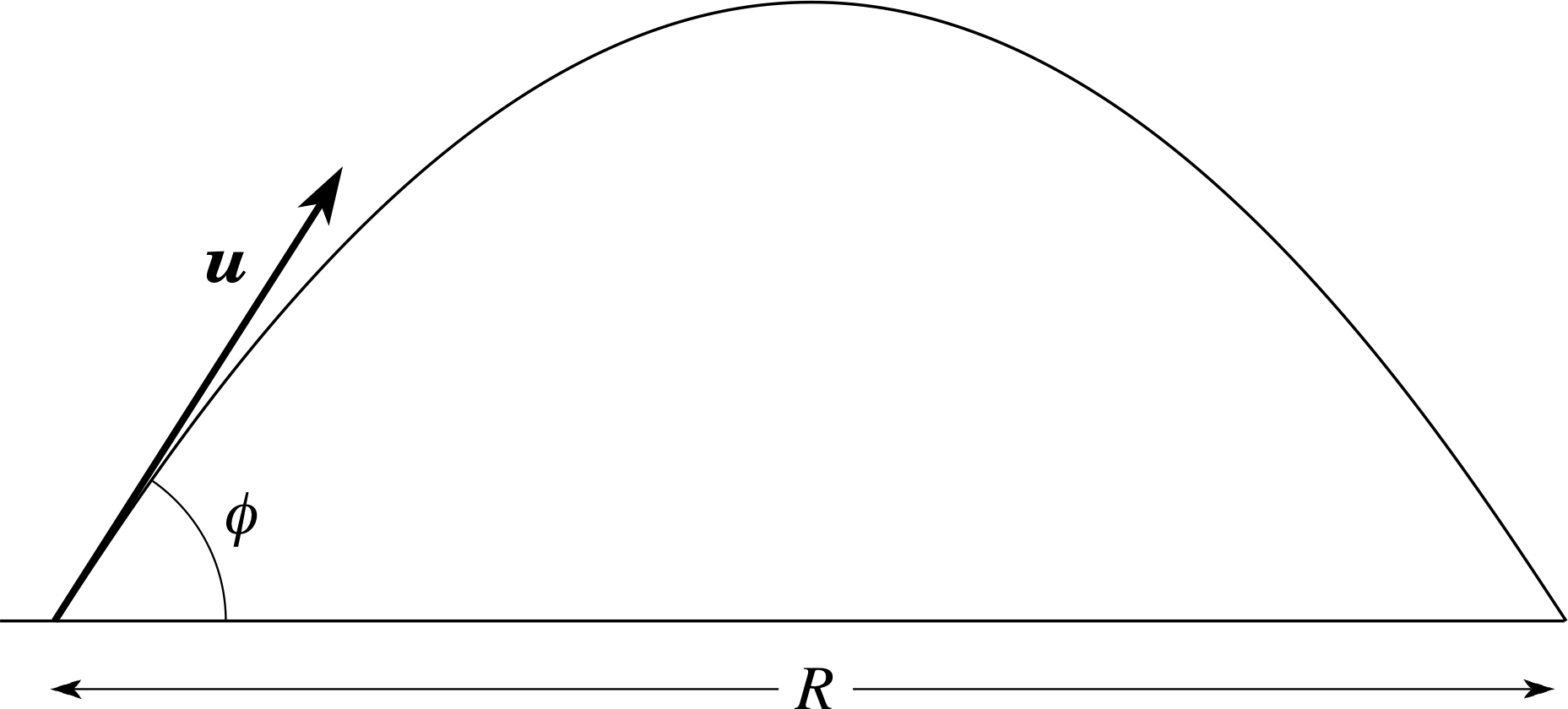
Figure 9 The range of a thrown ball.
$s_x = \dfrac{2u_y u_x}{g}$
This value of sx is the horizontal displacement from the point of projection (the launch) to the landing point.
The magnitude of this displacement is the range R. Therefore
$R = \left\lvert\,\dfrac{2u_y u_x}{g}\,\right\rvert$(28) i
We are now in a position to consider a problem which is of interest to cricketers or rounders players. At what angle to the horizontal, ϕ, should a fielder throw a ball to achieve maximum range?
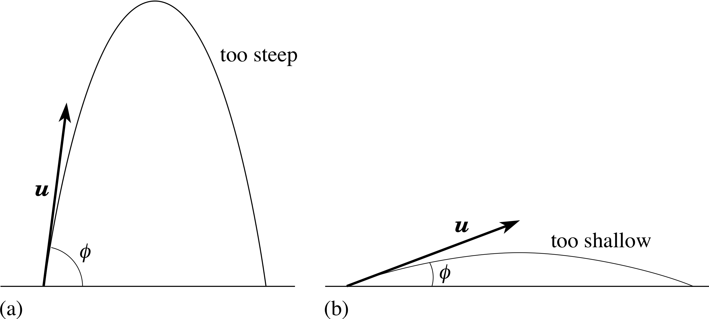
Figure 10 Maximizing the range of a projectile.
Figure 9 defines the range, while Figure 10 shows the effect on the range of varying the angle of projection. If the ball is thrown too steeply it achieves plenty of height but very little range. On the other hand, if it thrown at too shallow an angle, gravity will pull the ball down before it has chance to travel far. There must be some intermediate value of ϕ at which the maximum range is achieved.
To simplify the problem, we will assume that the ball is thrown from ground level at the same speed whatever the angle and that air resistance is negligible.
Suppose the ball is thrown with an initial velocity u at an angle ϕ to the horizontal, achieving a range R. The initial (and subsequent) horizontal component of velocity is ux = u cos ϕ and the initial vertical component of velocity is uy = u sin ϕ. Substituting these values into Equation 28 gives us
$R = \left\lvert\,\dfrac{2u^2\sin\phi\cos\phi}{g}\,\right\rvert$(29)
Using the trigonometric identity
2 sin ϕ cos ϕ = sin(2ϕ) i
Since u2 and g are positive quantities we can write Equation 29 as
$R = \dfrac{u^2}{g}\left \lvert\,\sin(2\phi)\,\right vert$(30) i
✦ Assuming ϕ is between 0° and 180°, what are the greatest and least values that sin(2ϕ) can have, and hence what is the maximum range?
✧ The maximum and minimum values of sin(2ϕ) are 1 and −1, respectively. In either case | sin(2ϕ) | = 1, so the maximum range is u2/g.
We now need to find the angle of projection, ϕ, which produces the maximum range.
✦ What is the value of ϕ that gives the maximum range? i
✧ If sin(2ϕ) = 1 then 2ϕ = 90°, and ϕ = 45°, or, if sin(2ϕ) = −1 then 2ϕ = 270°, and ϕ = 135°. Remember, ϕ is measured (anticlockwise) from the positive x–axis, so ϕ = 135° implies that the projectile is launched in the direction of the negative x– axis. In either case the projectile is launched at 45° to the horizontal.
A projectile moving near the Earth, under the influence of gravity alone, achieves maximum horizontal range when launched at 45° to the horizontal. i
For the flight of many objects, such as would be used in cricket or in putting the shot, these assumptions are fairly good.
Question T7
In the 1976 Olympic Games the shot–putting event was won with a throw of 21.32 m. Assuming that the shot was thrown from ground level at the optimum angle (45°), calculate the speed at which it was projected, making use of the formula for range. (Assume g = 9.81 m s−2).
Answer T7
We are given ϕ = 45° and range, R = 21.32 m. To find the initial speed of the throw we use
$R = \dfrac{u^2}{g}\left\lvert\,\sin(2\phi)\,\right|$(Eqn 30)
i.e.$u^2 = \dfrac{Rg}{\sin(2\phi)} = \rm \dfrac{21.32\,m\times 9.81\,m\,s^{-2}}{\sin 90°}$
thereforeu = 14.5 m s−1
In the next section you will learn how to solve similar problems in a more fundamental way, without resorting to the range formula.
4 Solving projectile problems
Using the ideas developed in the previous two sections you should be able to solve almost any projectile problem. It is particularly important to remember that:
In projectile motion, the horizontal component of velocity is constant and the vertical component of acceleration is constant. i
The usual strategy for dealing with projectile problems is as follows:
- 1
-
Express the initial velocity u in terms of its horizontal and vertical components ux = u cos ϕ and uy = u sin ϕ.
- 2
-
Treat each component of the motion as an example of one–dimensional (linear) motion: one along a horizontal line at a constant velocity, υx, and the other along a vertical line at a constant acceleration −g, (assuming vertically upwards to be the direction in which y increases).
- 3
-
Link the two component motions together by means of the total time of flight, T, which must be the same for each.
4.1 Some examples of projectile motion
Before you tackle a projectile problem on your own, here is a worked example.
Example 1
A cannon points at 60° above the horizontal and fires a ball from ground level with a muzzle speed of 20.0 m s−1. Find the horizontal range R, the maximum height h and the time of flight T. Neglect air resistance.
Solution
Using the strategy described above to solve this problem, we will first find the horizontal and vertical components of the initial velocity, ux and uy, respectively.
ux = (20.0 × cos 60°) m s−1 = 10.0 m s−1
anduy = (20.0 × sin 60°) m s−1 = 17.3 m s−1
We can now make use of the two properties of projectile motion.
Horizontal motion The displacement sx is given by Equation 17,
sx = uxt(Eqn 17)
The horizontal range R can be found from this equation by putting t = T, (where T denotes the time of flight) and taking the modulus.
ThereforeR = | uxT |(31)
We can find T by considering the vertical motion.
Vertical motion When the ball lands on the ground at the end of the flight t = T and the final vertical displacement is sy = 0. So, upon substituting sy = 0 and t = T into
sy = uyt − ½ gt2(20)
we have
0 = uyT − ½ gT 2 = T (uy− ½ gT)
This is a quadratic equation and therefore has two solutions. i These are
$T = 0 \quad\text{and}\quad T = \dfrac{2u_y}{g} = \rm \dfrac{2 \times 17.3\,m\,s^{-1}}{9.81\,m\,s^{-2}} = 3.53\,s$(32)
The first solution, T = 0, is the time the ball leaves the cannon; the second solution corresponds to the ball hitting the ground again and this is the time we need to find the range R.
Now that we have found the time of flight we can substitute this value for T into Equation 31,
R = | uxT |(Eqn 31)
giving R = | uxT | = 10 m s−1 × 3.53 s = 35.3 m. When the ball is at its maximum height, sy = h, and the vertical component of velocity is momentarily zero, so vy = 0. We can substitute these values into Equation 21,
υy2 = sy2 − 2gsy(Eqn 21)
to give the maximum height
0 = uy2− 2gh
i.e.$h = \dfrac{u_y^2}{2g} = \rm \dfrac{(17.3\,m\,s^{-1})^2}{2\times 9.81\,m\,s^{-2}} = 15.3\,m$
Now apply this strategy yourself to the next two questions.
Question T8
A cannon standing on the top of a cliff, 40 m high, fires a cannonball horizontally out to sea with a muzzle speed of 140 m s−1. How far out to sea does the ball go? (Assume g = 9.81 m s−2).
Answer T8
Since the cannonball is fired horizontally, the horizontal and vertical components of the initial velocity, uxand uy are, respectively,
ux = 140 m s−1 and uy = 0 m s−2
The horizontal motion is given by:
sy = uyt(Eqn 17)
So, if the time of flight is T and the range is R, we have
R = uyT
We can find T from the vertical motion:
The cannonball lands 40 m below the point of projection, therefore the vertical displacement, sx, at this point is −40 m and the time t = T.
If we use sy = uyt − ½ gt2(Eqn 20)
with uy = 0, we find
$T^2 = \dfrac{-2s_y}{g} = \rm \dfrac{8\,m}{9.81\,m\,s^{-2}}$
If we ignore the negative root, we find T = 2.86 s.
If we use this value of T in the equation for the range, we find the range out to sea is
R = uxT = 140 m s−1 × 2.86 s = 400 m.
Question T9
A golf ball is hit on level ground so that it leaves the ground with an initial velocity of 40.0 m s−1 at 30° above the horizontal. Find the greatest height reached by the ball, the total time of flight of the ball and the range of the shot. Neglect air resistance and assume g = 9.81 m s−2.
Answer T9
The horizontal and vertical components of the initial velocity are, respectively
ux = (40 × cos 30°) m s−1 and uy = (40 × sin 30°) m s−1
For the vertical motion, the greatest height is the value of sywhen υy = 0 m s−1.
From υy2 = uy2 − 2gsy(Eqn 21)
we have $\dfrac{u_y^2-\upsilon_y^2}{2g} = \rm \dfrac{(40\sin 30°\,m\,s^{-2})^2}{2\times 9.81\,m\,s^{-2}} = 20.4\,m$
To find the total time of flight, T, we use Equation 20,
sy = uyt − ½ gt2(Eqn 20)
and the fact that the displacement, sy, is zero on landing. Discarding the solution T = 0 gives us
$T = \dfrac{u_y}{g} = \rm \dfrac{(80\sin 30°)\,m\,s^{-1}}{9.81\,m\,s^{-2}} = 4.08\,s$
Considering the horizontal motion, the range R is given by the horizontal displacement, sx, at time T = 4.08 s.
From sx = uxt(Eqn 17)
we findR = uxT = (40 × cos 30°) m s−1 × 4.08 s = 141 m
(Since the launch and landing heights are the same, this problem could also be solved using the range formulae in Subsection 3.4).
4.2 The vector equations for motion with uniform acceleration
Study comment This subsection develops vector expressions for the equations of motion of a projectile. Familiarity with these expressions is not necessary in order to meet the achievements of this module, but they may help you to become more familiar with the use of vectors.
As indicated earlier, the methods developed in this module cannot only solve projectile problems, but any problem involving motion in two dimensions in which there is constant acceleration (including zero acceleration). So far, we have always chosen our axes so that there is no acceleration in the x–direction, and consequently ax = 0. When dealing with the general vector equations of uniformly accelerated two–dimensional motion, it does no harm to consider a more general case in which the x– and y–axes point in arbitrary directions in the plane of motion. In this general, case there will be uniform acceleration along both axes, so applying Equations 22, 23 and 24 in each case
υx = ux + axt(33)
andυy = uy + ayt(Eqn 22) i
We can write these as a single vector equation by using the rules for adding and scaling vectors that were introduced in Subsection 2.1
υ = (υx, υy) = (ux + axt, uy + ayt) = (ux, uy ) + (ax, ay)t
i.e. υ = u + at(34)
and in the same way we can write
sx = uxt + ½ axt2(35)
andsy = uyt + ½ ayt2(Eqn 23)
as the single vector equation s = ut + ½ at2(36)
The two–component equations
υx2 = ux2 + 2axsx(37)
and υy2 = uy2 + 2aysy(Eqn 24)
can be summed to give
υ2 = υx2 + υy2 = ux2 + uy2 + 2 (axsx + aysy)
which can be combined into a single equation
υ2 = u2 + 2a ⋅ s(38)
where the symbol a ⋅ s represents the scalar product of the vectors a and s which (in two dimensions) is defined by
a ⋅ s = axsx + aysy i
Note that it follows from this definition that the scalar product of two vectors is a scalar, so that Equation 38 is actually a scalar equation even though it is expressed in terms of vectors. It is also worth noting that the squared magnitudes υ2 and u2 that appear in Equation 38 could both be expressed as scalar products since
υ2 = υx2 + υy2 = (υ ⋅ υ) and u2 = ux2 + uy2 = (u ⋅ u)
υ = u + at(Eqn 34)
s = ut + ½ at2(Eqn 36)
Now, Equations 34, 36 and 38 are not frequently used, indeed Equation 38 actually scrambles together some of the information that is contained in Equations 24 and 37,
υx2 = ux2 + 2axsx(37)
andυy2 = uy2 + 2aysy(Eqn 24)
Nonetheless, the vector equations do emphasize the remarkable power of vectors. In particular, if we were asked to solve a three–dimensional problem in which a particle was free to move with components in three independent directions simultaneously (call them x, y and z), subject to constant acceleration in any direction, we could immediately say that Equations 34, 36 and 38 will describe the motion provided we interpret s, u, υ and a as three-dimensional vectors which can be represented by ordered triples such as s = (sx, sy, sz), u = (ux, uy, uz) and so on, and a ⋅ s is the three-dimensional scalar product defined by
a ⋅ s = axsx + aysy + azsz
So, vectors make it easy to write results in a form that is readily generalized to the three dimensions of the real world and are therefore of great value in physics.
Question T10
A puck is moving along the y–axis on an ice–rink (so that friction is negligible) at a speed of 10 m s−1. We define the y–axis along the surface of the rink, in the direction of the original motion of the puck. The x–axis is also on the surface of the rink and perpendicular to the y–axis. If the puck is subjected to an acceleration a = (2 m s−2, 0, 0) for 5 s, in what direction will it finally be moving? At the end of the acceleration, what is the displacement of the puck from its position at the start of the acceleration?
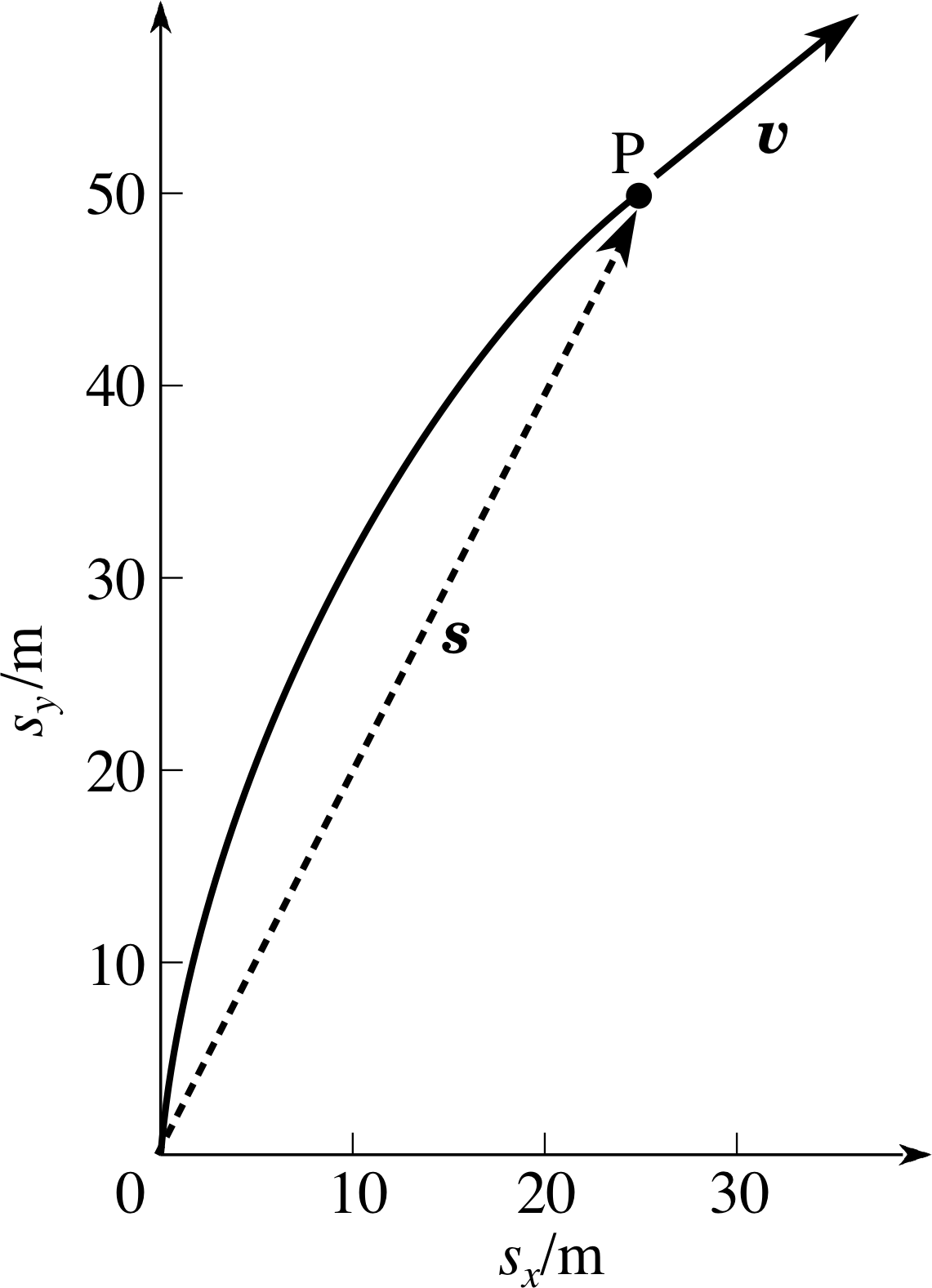
Figure 14 See Answer T10.
Answer T10
In this case it is the motion in the y–direction that is the uniform motion, and the motion in the x–direction that requires the use of the uniform acceleration equations. So we have
υx = ux+ axt = 0 + (2 m s−1) × (5 s) = 10 m s−1 and υx = 10 m s−1
So after 5 s the puck is at point P on Figure 14, moving at ϕ = arctan(10/10) = 45° to the x–axis.
Also, at this time
sx = uxt + ½ axt2 = 0 + ½ × 2 m s−2 × (5s)2 = 25 m
sy = uyt = 10 m s−1 × 5s = 50 m
In Figure 14 the trajectory is shown as a full line and its displacement after 5 s is shown as a dotted line from the initial position to point P. Note that the puck does not travel in a straight line from the starting point, even though its displacement after 5 s is shown as a straight line. Also note that the angles to the x–axis of the displacement s and velocity vector υ after 5 s are clearly different.
4.3 Solution to the introductory problem
Study comment This subsection contains the solution to the problem that was posed in Subsection 1.1. You should reread the problem and attempt to answer it before you work through the solution below.
We require the minimum muzzle speed. This corresponds to the launch velocity that will just enable the shell to reach the height of the aircraft. This means that the shell’s maximum height must equal the height at which the aircraft is flying. Since the shell is fired when the aircraft is directly overhead, the horizontal component of the muzzle velocity must equal the horizontal velocity of the aircraft, so that it arrives at the aircraft’s height with the correct horizontal displacement.
First consider the vertical motion. The vertical component of the initial velocity, uy is u sin ϕ and the vertical acceleration, ay is −9.81 m s−2. At the top point of the motion the displacement, sy is 2000 m and the vertical component of velocity, υy is 0 m s−1.
Using Equation 21,
υy2 = sy2 − 2gsy(Eqn 21)
we have 0 = u2 sin2 ϕ − 2gsy
so u2 sin2ϕ = 2gsy = 2 × 9.81 m s−2 × 2000 m = 3.92 × 10⁴(m s−1)2(39)
Now consider the horizontal motion. The horizontal constant velocity, υx is equal to the horizontal component of the launch velocity, that is u cos ϕ. To keep pace with the aircraft this must equal 150 m s−1.
Thereforeu cos ϕ = 150 m s−1
andu2 cos2 ϕ = 2.25 × 10⁴(m s−1)2(40)
If we add Equations 39 and 40 we obtain
u2(sin2ϕ + cos2ϕ) = (3.92 + 2.25) × 104(m s−1)2
Using the trigonometric identity sin2ϕ + cos2ϕ = 1
we findu2 = 6.17 × 10⁴(m s−1)2
sou = 248 m s−1
Now we need to find the launch angle ϕ. If we divide each side of Equation 39 by the corresponding side of Equation 40 we find:
$\dfrac{\sin^2\phi}{\cos^2\phi} = \tan^2\phi = \rm \dfrac{3.92 \times 10^4\,(m\,s^{-1})^2}{(2.25\times10^4\,(m\,s^{-1})^2)} = 1.74$
which gives ϕ = arctan(1.32) = 52.9°
For the shell to hit the aircraft, it should be fired with a minimum speed of 248 m s−1 (at an angle of 52.9° to the horizontal). It is worth noting that since υx is equal to the speed of the aircraft, the shell will be travelling vertically beneath the plane until it hits! On impact, the velocities of aircraft and shell will be identical (υx = 150 m s−1, υy = 0) and so the relative velocity between the two will be zero. Any damage to the aircraft will be due to the explosive charge, not the impact itself.
5 Closing items
5.1 Module summary
- 1
-
A projectile is an object that is launched into unpowered flight near the Earth’s surface.
- 2
-
Some projectiles can be adequately represented by point particles that move under the influence of gravity alone. In this approximation the flight of a projectile is an example of two-dimensional motion under constant acceleration.
- 3
-
The location of a point in a plane can be specified by its ordered pairposition coordinates (x, y) relative to a two–dimensional Cartesian coordinate system, or by its two–dimensional position vector, r. The position vector of a point can be specified in terms of its magnitude r = | r | (which represents the distance from the origin to the point) and its direction as given by the angle θ measured anticlockwise from the positive x–axis to r. The position vector of a point can also be specified in terms of its components which are equal to the position coordinates of the point, thus we can write r = (x, y) with $r = \lvert\,\boldsymbol{r}\,\rvert = \sqrt{x^2+y^2}$ and tan θ = y/x.
- 4
-
The displacement from a point with position vector r1 = (x1, y1) to a point with position vector r2 = (x2, y2) is defined by the vector quantity s = r2 − r1 = (x2 − x1, y2 − y1) and represents a change or difference in position. Unlike position vectors, displacements in a given system of coordinates are independent of any particular origin and may be measured from any selected reference point. In projectile motion the displacement of the projectile is usually measured from its launch point.
- 5
-
In general, vector quantities require both a magnitude and a direction for their complete specification and may be contrasted with scalar quantities which can be specified by a magnitude alone. In two–dimensions any vector υ may be represented by an ordered pair of (scalar) components (υx, υy); the magnitude of υ may then be written $\upsilon = \lvert\,\boldsymbol{\upsilon}\,\rvert = \sqrt{\upsilon_x^2+\upsilon_y^2}$, and its direction may be specified by the angle ϕ given by tan ϕ = υy /υx. Under these circumstances υx = υ cos ϕ and υy = υ sin ϕ.
- 6
-
Given two vectors of similar type the operation of vector addition allows us to add them graphically using the triangle rule or algebraically using
a + b = (ax, ay) + (bx, by) = (ax + bx, ay + by)(Eqn 7)
The operation of scaling allows us to multiply any vector by a scalar to produce another vector according to
λa = λ (ax, ay) = (λax, λay)(Eqn 8)
This has magnitude | λ | | a | and points in the same direction as a if λ is positive, and in the opposite direction if λ is negative.
- 7
-
The velocity, υ, and acceleration, a, of a particle moving in two dimensions are vector quantities that are defined as follows:
${\boldsymbol\upsilon} = (\upsilon_x,\,\upsilon_y) = \dfrac{d{\boldsymbol{ r}}}{dt} = \left(\dfrac{dx}{dt},\,\dfrac{dy}{dt}\right)$(Eqn 12)
${\boldsymbol a} = (a_x,\,a_y) = \dfrac{d\boldsymbol \upsilon}{dt} = \left(\dfrac{d\upsilon_x}{dt},\,\dfrac{d\upsilon}{dt}\right)$(Eqn 13)
The magnitude of the velocity is called the speed and cannot be negative.
- 8
-
Projectile motion is characterized by a constant horizontal velocity component, υx = ux, and a constant vertical acceleration component, ay, the magnitude of which is equal to the magnitude of the acceleration due to gravity, g. i
- 9
-
Uniform motion equations may be applied to the horizontal motion of a projectile, giving
sx = uxt(Eqn 17)
υx = ux = constant(Eqn 16)
andax = 0(Eqn 15)
where the displacement, sx, is taken to be zero when t = 0.
- 10
-
Uniform acceleration equations may be applied to the vertical motion of a projectile, giving
υy = uy − gt(Eqn 19)
sy = uyt − ½ gt2(Eqn 20)
υy2 = sy2 − 2gsy(Eqn 21)
where the y–axis has been assumed to point vertically upwards and the displacement, sy, is taken to be zero when t = 0.
- 11
-
A projectile moving near the Earth, under the influence of gravity alone, follows a parabolic trajectory and achieves maximum horizontal range when launched at 45° to the horizontal.
- 12
-
The strategy used to solve projectile problems is to resolve the initial velocity into its horizontal and vertical components and subsequently to treat each component as an example of linear motion.
- 13
-
Similar principles and methods apply whenever a particle is subject to constant acceleration in a direction other than its direction of motion, or opposite to this direction.
- 14
-
Vector methods of the sort developed to treat two–dimensional projectile problems may be readily extended to deal with three-dimensional problems
5.2 Achievements
Having completed this module, you should be able to:
- A1
-
Define the terms that are emboldened and flagged in the margins of the module.
- A2
-
Describe in quantitative terms the magnitude and direction of two–dimensional vector quantities such as displacement, velocity and acceleration given their horizontal and vertical components.
- A3
-
Draw and interpret graphical representations of vector quantities such as the position, displacement and velocity of a projectile.
- A4
-
Recall and apply the equations of motion that describe the behaviour of projectiles. (Equations 15–21 for motion under gravity, and Equations 2 – 4 more generally.)
- A5
-
Solve problems concerning the range, time of flight, maximum height, velocity and displacement of projectiles.
- A6
-
Solve general problems involving two–dimensional motion with uniform acceleration.
Study comment You may now wish to take the following Exit test for this module which tests these Achievements. If you prefer to study the module further before taking this test then return to the topModule contents to review some of the topics.
5.3 Exit test
Study comment Having completed this module, you should be able to answer the following questions, each of which tests one or more of the Achievements. i
Question E1 (A3)
Sketch a Cartesian coordinate system, showing the origin and the point with position vector r = (1 m, 2 m). What is the distance of this point from the origin?
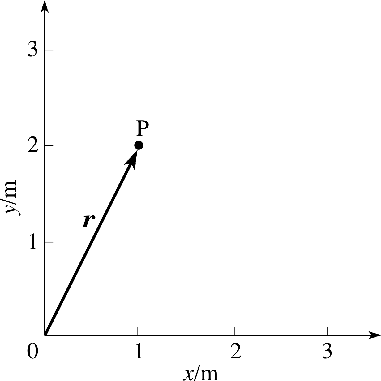
Figure 15 See Question E1.
Answer E1
Figure 15 illustrates the point P located by the position vector (1 m, 2 m). The distance from the origin O to the point marked is given by the magnitude, r, of the position vector r:
$r = \sqrt{x^2 + y^2} = \rm \sqrt{1^2 + 2^2}\,m = 2.24\,m$
(Reread Subsection 2.1 if you had difficulty with this question.)
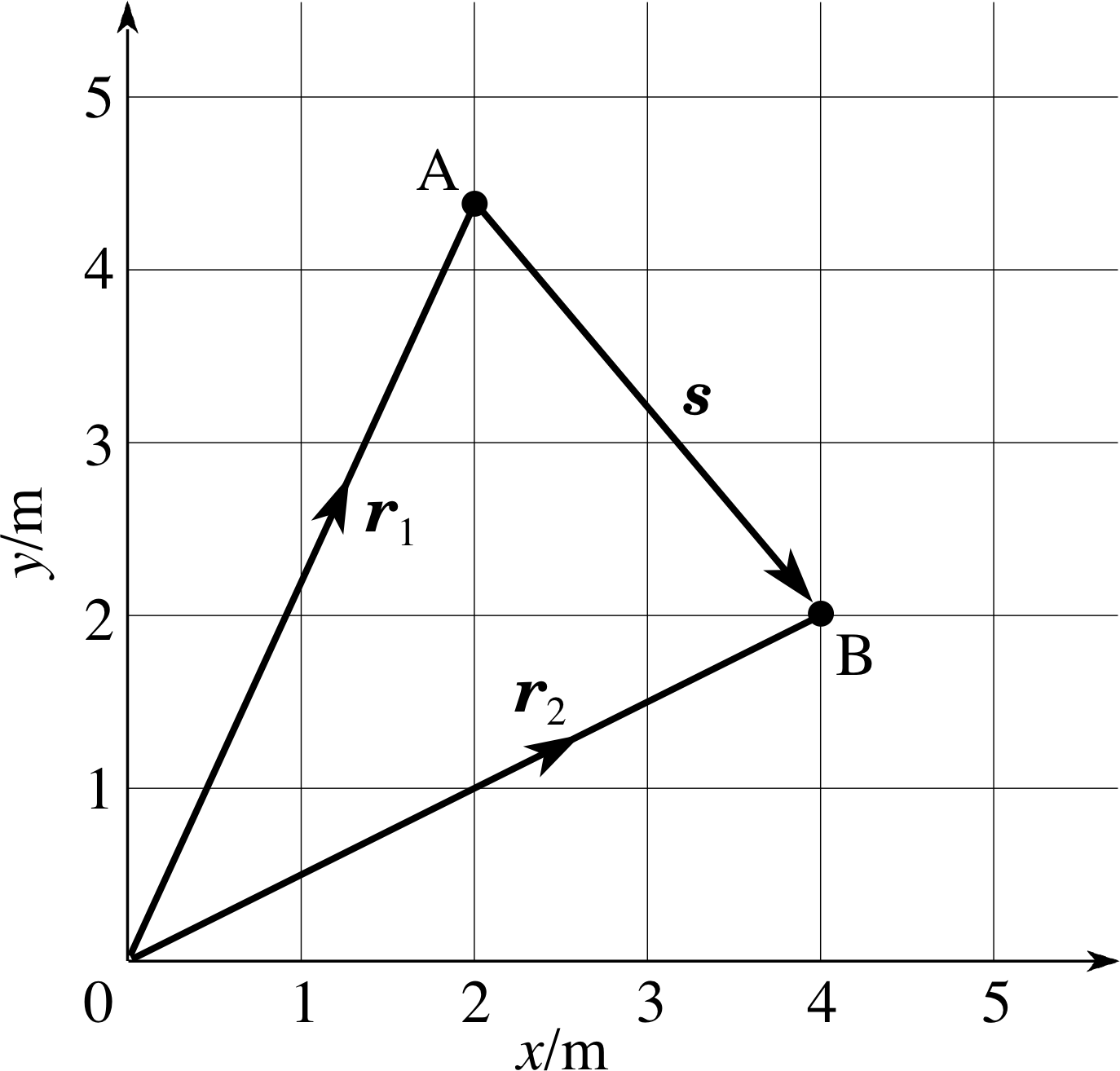
Figure 11 See Question E2.
Question E2 (A2 and A3)
A ball is at point A in Figure 11 at a time t1 = 1.4 s and at point B at a time t2 = 1.8 s. Find the displacement from A to B and hence find the average velocity vector over the time interval from t = 1.4 s to t = 1.8 s.
Answer E2
The displacement:
s = r2 − r1 = (∆x, ∆y)
s = (4.0 m − 2.0 m, 2.0 m − 4.4 m) = (2.0 m, −2.4 m)
The average velocity vector is the rate of change of displacement:
$\langle \upsilon \rangle = \left(\dfrac{\Delta x}{\Delta t},\,\dfrac{\Delta y}{\Delta t}\right) = \rm \left(\dfrac{2.0\,m}{0.4\,s}\right),\,\left(\dfrac{-2.4\,m}{0.4\,s}\right) = (5.0\,m\,s^{-1},\,-6.0\,m\,s^{-1})$
(Reread Subsection 2.1 if you had difficulty with this question.)
Question E3 (A3, A4 and A5)
The opening to a basketball net is 3.05 m above the ground. A player’s feet are 6 m away from a mark on the floor immediately below the net. The player throws the basketball from a height of 2 m and at an angle of 60° above the horizontal. With what speed should the player throw the ball in order to get it into the net? (Assume g = 9.81 m s−2, and that both the ball and net can be treated as point objects.)
Answer E3
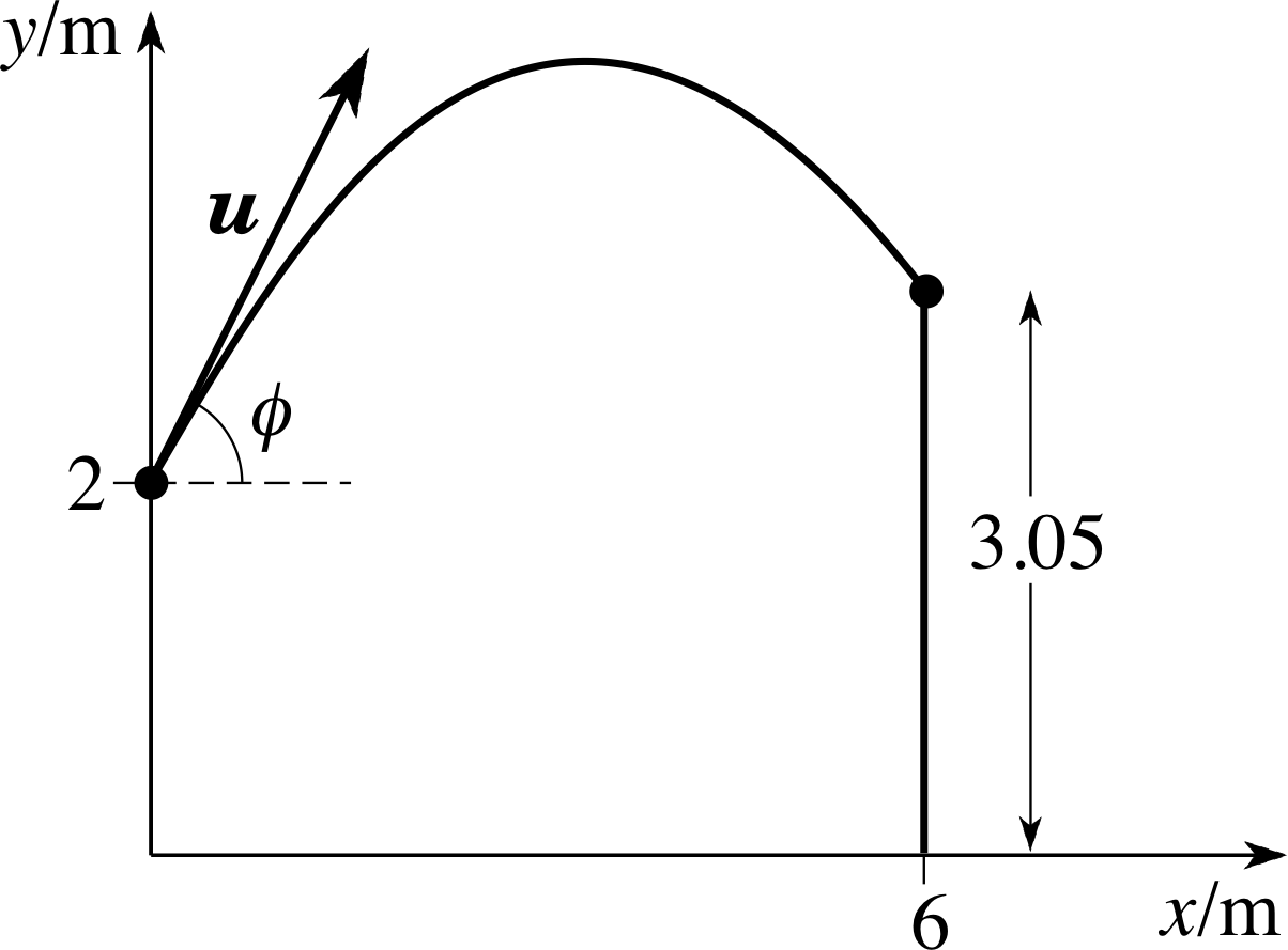
Figure 16 See Question E3.
Figure 16 summarizes the information given in the question.
The minimum value for the vertical displacement sy = 1.05 m.
For the horizontal motion:
sx = 6 m and ux = u cos 60° = u/2
To find the time, t, to travel a horizontal distance of 6 m we use
sx = uxt(Eqn 17)
$t = \dfrac{s_x}{u_x} = \dfrac{2s_x}{u}$
For the vertical motion:
sy = 1.05 m (from the launch point), $u_y = u\sin 60° = u\sqrt{3\os}/2$
Substituting for t = 2sx /u in Equation 20,
sy = uyt − ½ gt2(Eqn 20)
we find$s_y = \dfrac{u\sqrt{3\os}\times 2s_x}{2u} - \dfrac{g}{2}\times \dfrac{4s_x^2}{u^2}$
i.e.$\dfrac{2gs_x^2}{u^2} = s_x\sqrt{3\os} - s_y$
So$u^2 = \dfrac{2gs_x^2}{(s_x\sqrt{3\os}-s_y)} = \rm \dfrac{2\times 9.81\,m\,s^{-2}\times (6\,m)^2}{(6\times \sqrt{3\os}-1.05)\,m} = 75.6\,m^2\,s^{-2}$ and u = 8.70 m s−1
(Reread Section 3 if you had difficulty with this question.)
Question E4 (A4 and A5)
A rifleman holds his rifle with its barrel horizontal at a height of 1.5 m above the ground. He is aiming at the centre of a target which is 100 m away and also at a height of 1.5 m. Assuming the muzzle speed of the bullet to be 500 m s−1, and that the barrel is lined up with the target, find the time taken for the bullet to reach the target and the vertical distance by which the bullet will miss the centre of the target. Take g = 9.81 m s−2.
Answer E4
For the horizontal motion:
ux = 500 m s−1 and sx = 100 m
The time taken for the bullet to reach the target is given by
sx = uxt(Eqn 17)
i.e.$t = \dfrac{s_x}{u_x} = \rm \dfrac{100\,m}{500\,m\,s^{-1}} = 0.20\,s$
For the vertical motion:
We know that the vertical component of the initial velocity, uy = 0 m s−1. The vertical displacement, sy, from the starting point at the time, t = 0.20 s is given by
sy = uyt − ½ gt2(Eqn 20)
i.e.sy = −½ × 9.8 ms−2 × (0.2 s)2 = −0.2 m (to two significant figures)
The bullet will arrive 0.20 m below the centre of the target.
(Reread Subsections 3.1 and 3.2 if you had difficulty with this question.)
Question E5 (A4 and A5)
A stone is thrown horizontally from the top of a vertical cliff with a velocity of 15 m s−1. It is observed to reach the sea at a point 45 m from the foot of the cliff. Find the time of flight of the stone and the height of the cliff.
Answer E5
For the horizontal motion:
ux = 15 m s−1 and sx = 45 m
The time of travel, t, is found from
sx = uxt(Eqn 17)
$t = \dfrac{s_x}{u_x} = \rm \dfrac{45\,m}{15\,m\,s^{-1}} = 3.0\,s$
For the vertical motion:
The height of the cliff, which is numerically equal to the vertical displacement, sy, after 3.0 s may be found using
sy = uyt − ½ gt2(Eqn 20)
with t = 3.0 s and uy = 0 m s−1
sosy = 0 m − ½ × 9.8 ms−2 × (3.0 s)2 = −44.1 m
So the height of the cliff is 44 m (two significant figures).
(Reread Subsection 3.2 if you had difficulty with this question.)
Question E6 (A3, A4 and A5)
A gun fires shells from ground level with a muzzle speed of 300 m s−1. In a test, shells are fired at (a) 30°, (b) 45° and (c) 60° to the horizontal. Assuming that g = 9.81 m s−2 find the range and the maximum height reached for each angle of firing. Using centimetre–squared graph paper, sketch a scale drawing of each trajectory using the same set of axes.
Answer E6
For an angle of projection of ϕ, the horizontal component of initial velocity is given by, ux = 300 cos ϕ and the vertical component is given by, uy = 300 sin ϕ.
For the vertical motion:
We can find the maximum height reached by using Equation 21,
υy2 = uy2 − 2gsy(Eqn 21)
withυy = 0 m s−1 and sy = h
so$h = \dfrac{u_y^2}{2g} = \dfrac{(u\sin\phi)^2}{2g}$
When the shell lands, sy = 0 m, so we can use
sy = uyt − ½ gt2(Eqn 20)
to find the time of flight, at t = T. Therefore, ignoring the solution T = 0, the other solution is given by
$T = \dfrac{2u_y}{g} = \dfrac{2u\sin\phi}{g}$
For the horizontal motion:
In this case the range, R is equal to the horizontal displacement after a time T. We can use Equation 17,
sx = uxt(Eqn 17)
to give
R = uxT = uT cos ϕ
and so we find
$R = \dfrac{2u^2\cos\phi\sin\phi}{g} = \dfrac{u^2\sin(2\phi)}{g}$(Eqn 30)
We can now use the expressions for h and R to find these for each firing angle.
Figure 17 See Question E6.
(a) When ϕ = 30°
$h = \dfrac{(u\sin\phi)^2}{2g} = \rm \dfrac{[(300\sin30°)\,m\,s^{-1}]^2}{2 \times 9.81\,m\,s^{-2}} = 1.15\,km$
$R = \dfrac{u^2\sin(2\phi)}{g} = \rm \dfrac{(300\,m\,s^{-1})^2\sin 60°}{ 9.81\,m\,s^{-2}} = 7.95\,km$
Similar calculations lead to the maximum height and the range for a shell projected at angles of 45° and 60° to the horizontal as:
(b) 45° to the horizontal: h = 2.29 km and R = 9.17 km
(c) 60° to the horizontal: h = 3.44 km and R = 7.95 km
Figure 17 illustrates these three trajectories.
(Reread Subsection 3.4 if you had difficulty with this question.)
Question E7 (A4 and A5)
Look back at the information given in Question T7
In the 1976 Olympic Games the shot–putting event was won with a throw of 21.32 m. Assuming that the shot was thrown from ground level at the optimum angle (45°), calculate the speed at which it was projected, making use of the formula for range. (Assume g = 9.81 m s−2).
and recalculate the speed needed on the assumption that the shot was launched at 45°, but from a height of 2 m rather than from ground level.
Answer E7
Since the launch height differs from the landing height we cannot now use the range formula given in Equation 30. We must solve the problem directly from the equations of motion. We set the new launch speed = u.
At launch we have: ux = u cos 45° = $\dfrac{u\sqrt{2\os}}{2}\quad\text{and}\quad u_y = u\sin 45° = \dfrac{u\sqrt{2\os}}{2}$
At landing: sy = −2 m (measured from the launch position) and sx = 21.32 m.
The time of flight can be found from:
$T = \dfrac{s_x}{u_x} = \dfrac{2s_x}{u\sqrt{2\os}}$
and using Equation 20,
sy = uyt − ½ gt2(Eqn 20)
we obtain
$s_y = \dfrac{u\sqrt{2\os}}{2} \times \dfrac{2s_x}{u\sqrt{2\os}} - \dfrac{g}{2} \times \dfrac{4s_x^2}{2u^2}$
so$s_y = s_x - g\dfrac{s_x^2}{u^2}$
Therefore$u^2 = \dfrac{gs_x^2}{s_x-s_y} = \rm \dfrac{9.81\,m\,s^{-2}\times(21.32\,m)^2}{23.32\,m} = 191.2\,(m\,s^{-1})^2$
i.e.u = 13.8 m s−1 which is, as expected, slightly less than our earlier calculation of 14.5 m s−1 in Question T7.
(Reread Section 4 if you had difficulty with this question.)
Question E8 (A4 and A6)
An ice puck is travelling along the y–axis of the rink at 2 m s−1. At a particular instant, when its position coordinates are (x, y) = (0 m, 5 m), it begins to accelerate parallel to the x–axis with ax = 2 m s−2. Find its new position and velocity vectors after 5 s, and express each of these in both component and magnitude/direction notation.
Answer E8
We have uy = 2 m s−1 and ay = 0.
At the moment when acceleration begins, ux = 0 and ax = 2 m s−2.
When T = 5 s the y–displacement is
sy = uyT = 2 m s−1 × 5 s = 10 m
The x–displacement, using Equation 23 (suitably reinterpreted), is
s x = ux T + ½ axT 2
These displacements are measured from the initial position (0 m, 5 m), therefore
sx = ½ (2 m s−2)(5 s)2 = 25 m
The position coordinate after 5 s is thus (0 m + 25 m, 5 m + 10 m), i.e. (25 m, 15 m). The new position r can be characterized either in terms of its components or its magnitude and direction. In terms of components, this position is r = (x, y) = (25 m, 15 m), i.e. it has a magnitude of r = (x2 + y2)1/2 = (252 + 152)1/2 m = 29.2 m at an angle to the x–axis, θ = arctan( y/x) = arctan(15/25) = 31.0°.
The velocity components after 5 s are:
υx = ux + axt = 0 + 2 m s−2 × 5 s = 10 m s−1
andυy = uy = 2 m s−1
The final velocity vector υ = (10 m s−1, 2 m s−1), it has magnitude of υ = (υx2 + υy2)1/2 = (102 + 22)1/2 m s−1 = 10.2 m s−1 and an angle to the x–axis
ϕ = arctan(υy /υx) = arctan(2/10) = 11.3°
Notice that ϕ and θ are quite different.
(Reread Subsection 4.2 if you had difficulty with this question.)
Study comment This is the final Exit test question. When you have completed the Exit test go back and try the Subsection 1.2Fast track questions if you have not already done so.
If you have completed both the Fast track questions and the Exit test, then you have finished the module and may leave it here.
Study comment Having seen the Fast track questions you may feel that it would be wiser to follow the normal route through the module and to proceed directly to the following Ready to study? Subsection.
Alternatively, you may still be sufficiently comfortable with the material covered by the module to proceed directly to the Section 5Closing items.