PHYS 4.2: Introducing magnetism |
PPLATO @ | |||||
PPLATO / FLAP (Flexible Learning Approach To Physics) |
||||||
|
1 Opening items
1.1 Module introduction
One of the simplest ways to demonstrate magnetism is to dip a magnet into a box of paper clips – with care, you may succeed in picking up 20 or 30 clips. The objects around us divide broadly into two groups: those which are attracted by a magnet and those which are not. Those attracted by a magnet are made of ferromagnetic materials. In the case of the paper clips, the property of magnetic attraction is transferred by magnetic induction from the magnet to the nearest clips, which themselves then act as magnets and attract further clips.
In Section 2 of this module, you will see how interactions between magnets are described in terms of magnetic poles and magnetic fields. You will learn how to plot magnetic field lines, using either iron filings or a compass needle, how to interpret such plots, and how to sketch the field lines of magnets in new orientations and positions. This section of the module also includes a discussion of magnetic dipoles and monopoles, and ends with an overview of magnetic properties of materials.
Section 3 describes how magnetic fields can also be produced by electric currents, as shown by Hans Christian Oersted (1777–1851) in 1820. This section then discusses the magnetic fields produced by electric currents in certain well–defined circuit configurations, namely a long straight wire, a circular loop of wire, a solenoid and a toroidal solenoid. Using the right-hand grip rule and the principle of superposition, it shows how the field patterns from more complicated current configurations can be built up. The formulae for the magnetic field strengths produced by these basic current configurations are given, allowing the numerical calculation of these field strengths in various situations.
Study comment Having read the introduction you may feel that you are already familiar with the material covered by this module and that you do not need to study it. If so, try the following Fast track questions. If not, proceed directly to the Subsection 1.3Ready to study? Subsection.
1.2 Fast track questions
Study comment Can you answer the following Fast track questions? If you answer the questions successfully you need only glance through the module before looking at the Subsection 4.1Module summary and the Subsection 4.2Achievements. If you are sure that you can meet each of these achievements, try the Subsection 4.3Exit test. If you have difficulty with only one or two of the questions you should follow the guidance given in the answers and read the relevant parts of the module. However, if you have difficulty with more than two of the Exit questions you are strongly advised to study the whole module.
Question F1
The Earth’s magnetic field is often described as being similar to that of a short bar magnet, placed near the centre of the Earth, with its south pole nearest the Earth’s geographic North Pole.
(a) How do you explain this apparent ambiguity in the use of north and south?
(b) What evidence supports the statement that an equivalent field would be produced by a short bar magnet?
(c) In what region(s) of the Earth would you expect to find no vertical component to the Earth’s field, i.e. a zero angle of dip?
Answer F1
(a) The north pole of a compass is that pole which is attracted towards the geographic North Pole of the Earth. Since unlike poles attract, then we must conclude that the Earth must have a south magnetic pole pointing towards the geographic North Pole and vice versa.
(b) Close to the north and south magnetic poles at the Earth’s surface, the magnetic field is nearly vertical. This can only arise if the Earth’s magnetic poles are deep lying, i.e. the poles of a short bar magnet the nearer the poles are to the surface, then the greater the departure from 90° of the angle of dip near the poles.
(c) Places with zero angle of dip would define a magnetic equator, and we would expect the Earth’s magnetic equator to coincide approximately with the geographic equator.
Question F2
You are given three apparently identical iron rods, but are told that two of them are permanently magnetized. How would you distinguish which two are the magnets?
Answer F2
Select two of the rods and bring an end of one towards an end of the other. If they repel each other, then you will know that they are both magnets, because repulsion can only occur between two like poles. If they attract each other, then reverse one of the rods so as to use the other end. If they now repel each other, then they are the magnets, and the unused rod is unmagnetized. If they still attract, you must have selected only one magnet, but you will not know which it is. To find out, take one of your selected pair and go through the same procedure using it and the third rod.
Question F3
Two concentric coils of wire are positioned with their planes perpendicular to one another. Coil A has 100 turns of radius 30 cm and carries a current of 1.5 A; coil B has 50 turns of radius 10 cm and a current of 0.9 A. Given that the magnitude of the field at the centre of a coil of N turns of radius R carrying a current I is given by B = μ0NI/(2R), where μ0 = 4π × 10−7 T m A−1, find the magnitude of the resultant magnetic field at the centre of the coils.
Answer F3
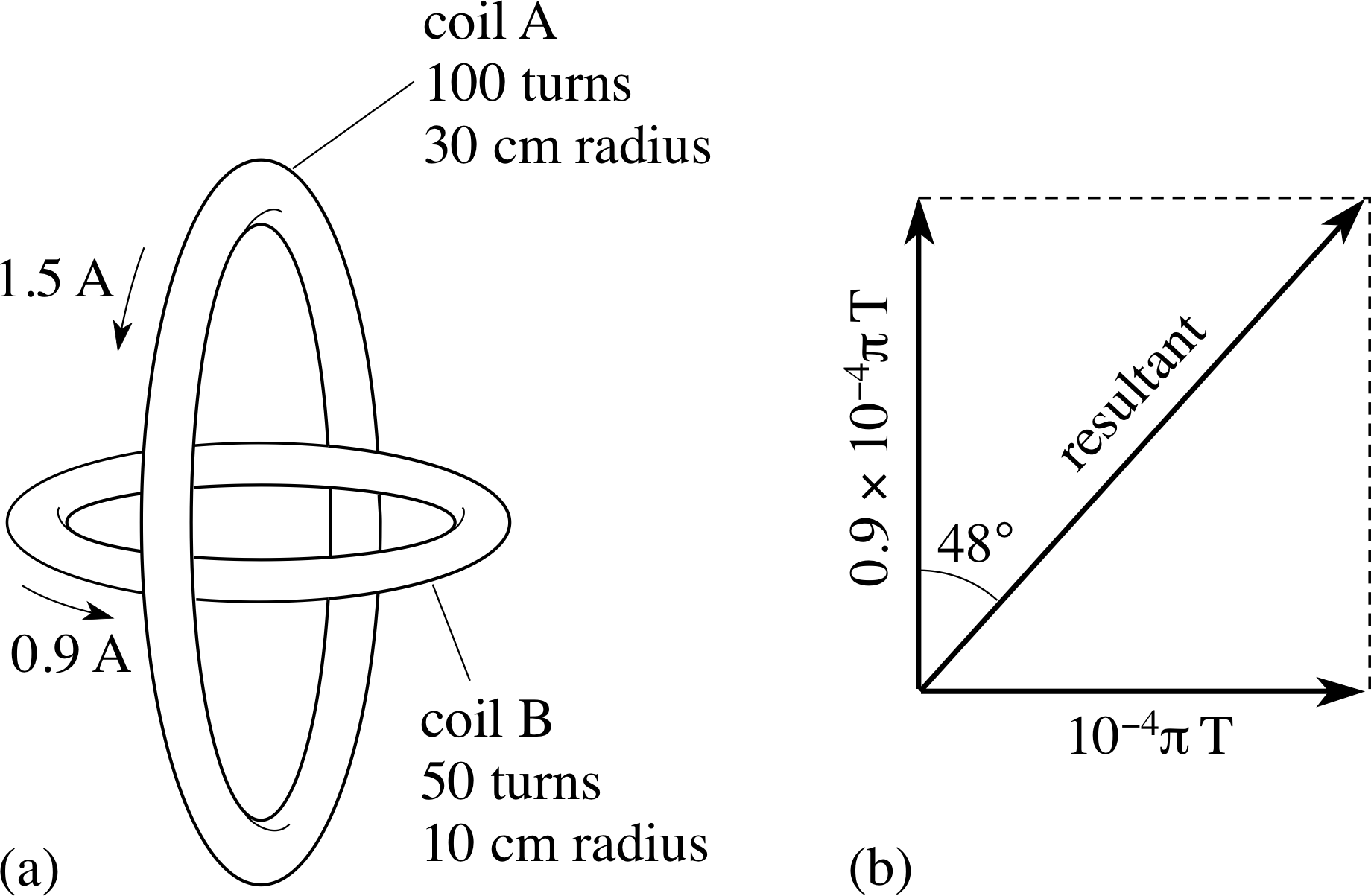
Figure 23 See Answer F3.
The arrangement of the two coils is shown in Figure 23a. The direction of the field produced at the centre of a coil is at right angles to the plane of the coil, therefore, as the coils are perpendicular, the fields they produce at their centres are also perpendicular. The strength of these fields are as follows:
$B_{\rm A} = \dfrac{4\pi\times 10^{-7}\,{\rm T\,m\,A^{-1}\times 100\times 1.5\,A}}{2\times 30\times 10^{-2}\,{\rm m}} = 10^{-4}\pi\,{\rm T}$
$B_{\rm B} = \dfrac{4\pi\times 10^{-7}\,{\rm T\,m\,A^{-1}\times 50\times 0.9\,A}}{2\times 10\times 10^{-2}\,{\rm m}} = 0.9\times 10^{-4}\pi\,{\rm T}$
These fields are as shown in Figure 23b (you may have these in different directions if the current in your coils were not the same as in (a), but your resultant field should still have the same magnitude).
When added together, the resultant field strength is
$B = \sqrt{(10^{-4}\pi)^2 + (0.9\times 10^{-4}\pi)^2}\,{\rm T} = 4.23\times 10^{-4}\,{\rm T}$
The resultant field is at an angle to the plane of the large coil whose tangent is BA/BB = 1/0.9, that is, an angle of 48°.
1.3 Ready to study?
Study comment In order to study this module you will need little background knowledge of magnetism, beyond its occurrence. The module is not mathematically demanding because the formulae associated with magnetic fields are quoted and not proved. You will however need to be familiar with the following terms: density, electric charge, electric current, energy, force, scalar, speed, temperature, vector, velocity and weight. You will also need to be familiar with vectorvector notation, including magnitude_of_a_vector_or_vector_quantitymagnitude of a vector, and the idea of combining vectors in one and two dimensions, using the triangle_ruletriangle or parallelogram_ruleparallelogram rules and simple trigonometry. If you are uncertain about any of these terms then you can review them now by reference to the Glossary, which will also indicate where in FLAP they are developed. The following questions will allow you to establish whether you need to review some of these topics before embarking on this module.
Question R1
Which of the following quantities are vectors and which are scalars: density, energy, force, speed, temperature, velocity and weight?
Answer R1
The vectors are: force, velocity and weight (which is a force). They all have direction as well as magnitude_of_a_vector_or_vector_quantitymagnitude. The scalars are: density, energy, speed (which is the magnitude of the velocity) and temperature. None of these has direction associated with it.
Consult vectors and scalars in the Glossary for further information.
Question R2
When an electric current flows in a copper wire, what type of charged particle moves in the wire to constitute that current? In what way does this movement differ from the electric_currentconventional current in the wire?
Answer R2
The current consists of a movement of electrons, which have negative charge. The electrons move away from the negative terminal of a power supply and towards the positive terminal. Historically however, an electric current was first defined as the movement of positively charged particles, i.e. towards the negative terminal of a power supply and away from the positive terminal – and this convention has remained. So we speak of the conventional current and think of this as consisting of positive particles flowing. In the case of current in a copper wire, a negative charge flowing in one direction is exactly equivalent (i.e. the same magnitude) to a positive charge flowing (i.e. a conventional current) in the opposite direction.
Consult electric current in the Glossary for further information.
Question R3
A particle is subjected to two forces, each of the same magnitude_of_a_vector_or_vector_quantitymagnitude F, acting simultaneously. Find the direction and magnitude of the resultant force in each of the following cases:
(a) both forces act in a northerly direction;
(b) one force acts in a northerly direction and the other in a southerly direction;
(c) one force acts in a northerly direction and the other in an easterly direction.
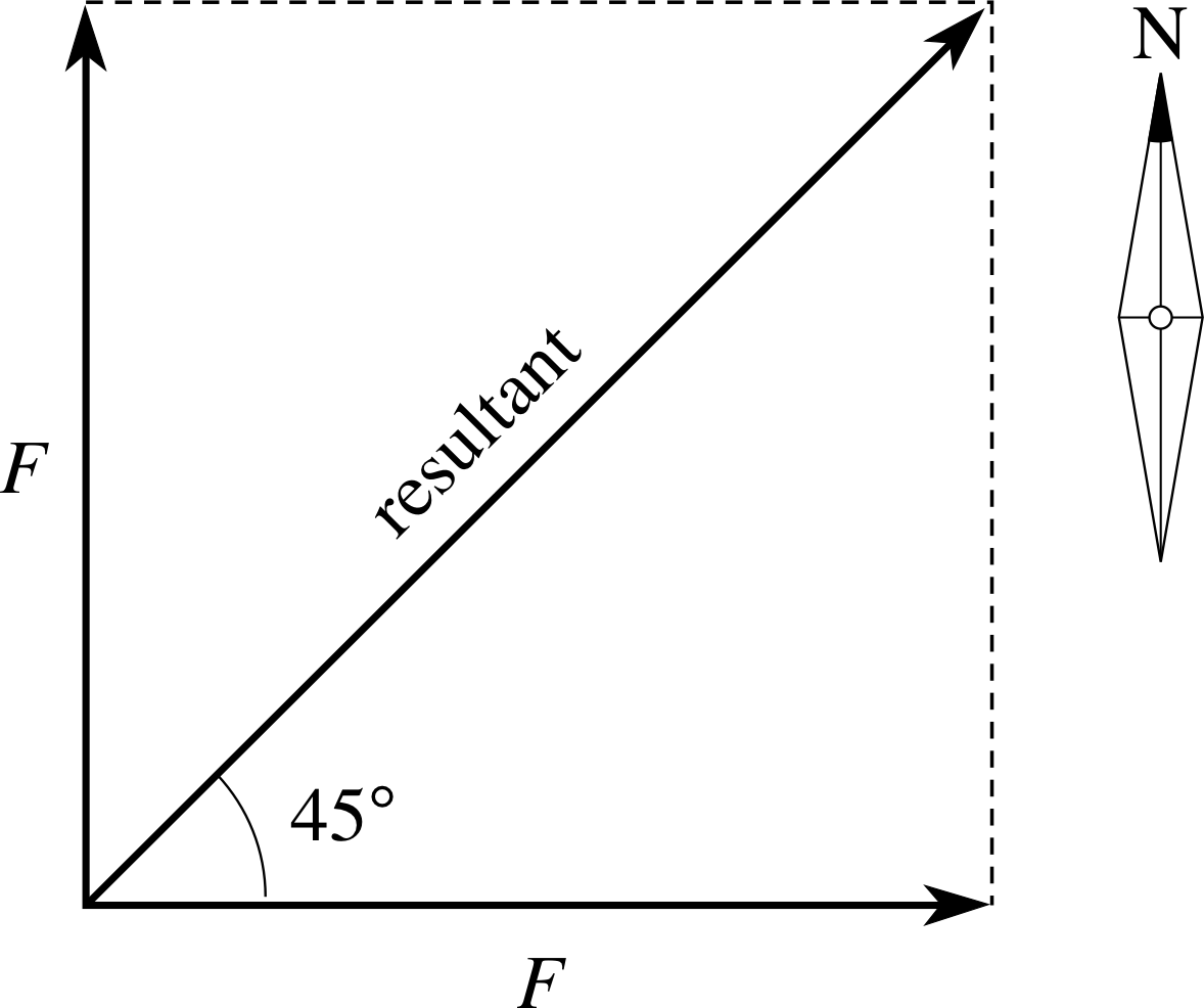
Figure 24 See Answer R3.
Answer R3
(a) A force of magnitude_of_a_vector_or_vector_quantitymagnitude 2F, acting in a northerly direction.
(b) Zero.
(c) The force acts in a north–easterly direction, and has magnitude $\sqrt{2\os} \times F$ (see Figure 24). This is an example of the resultant_vectorresultant of two forces of equal magnitude acting at right angles.
Consult vector addition in the Glossary for further information.
2 Magnets and magnetic fields
2.1 Magnetism in everyday life
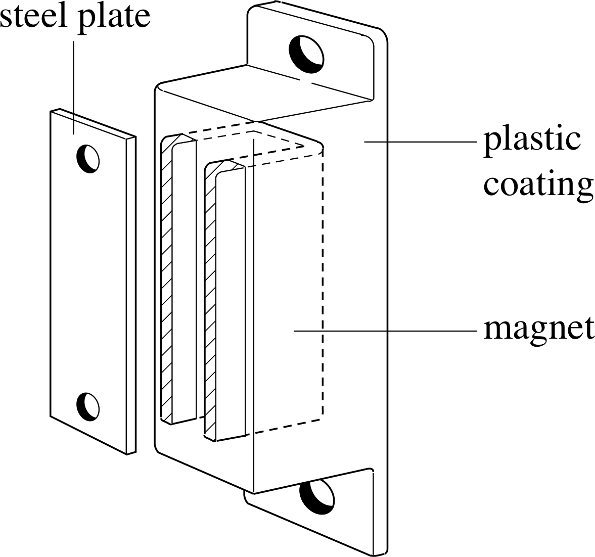
Figure 1 A magnetic cupboard catch.
Most of us are familiar with some simple applications of magnets and magnetism around the home which make use of the attractive force between small magnets and unmagnetized pieces of steel. i Magnetic cupboard catches (Figure 1) often consist of a small powerful horseshoe–shaped magnet attached to a door jamb, which exerts a strong retaining force on a steel plate attached to the door, when brought into contact. Many refrigerator doors are held closed by magnetic forces, though in this case the magnetized material, often a special ceramic powder, is dispersed in a rubber or plastic strip around the door opening and the steel of the door itself is attracted to the strip. Magnets are also to be found in television sets, electric motors, microwave ovens and loudspeakers.
A more ancient application of magnetism than any of the above examples can be seen in the compass. These small pivoted bar magnets have been used for navigation since the 11th century. The magnetic properties of certain minerals (e.g. magnetite or lodestone, containing the iron oxide Fe2O3), were known to the Greeks some 2300 years ago, and compass needles were once made by stroking (in one direction) a steel needle with a lodestone.
Magnetism may sometimes be seen in unexpected circumstances. Steel tools are sometimes found to have acquired magnetic properties, as shown by their ability to attract iron filings or small screws or nails – screwdrivers and cold chisels often exhibit this effect. i
2.2 Magnetic poles
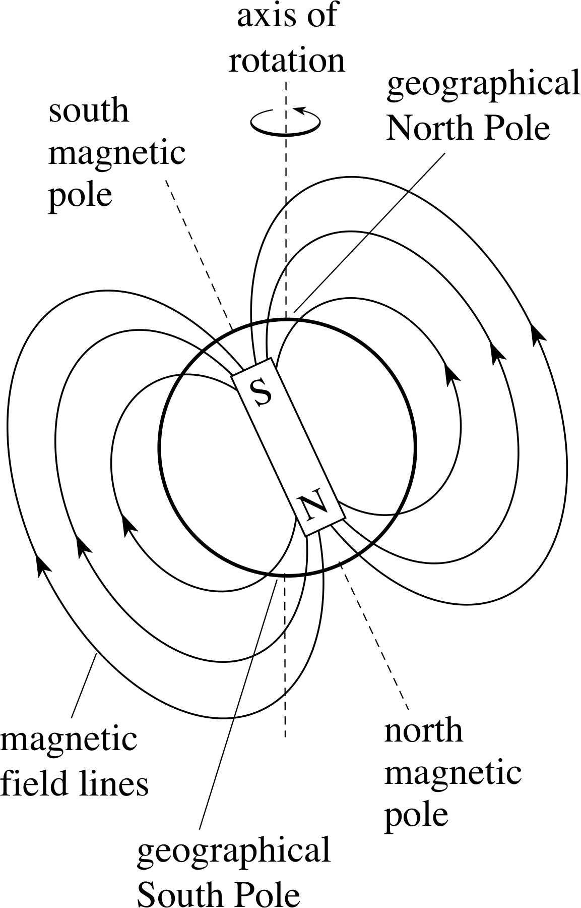
Figure 2 The Earth’s magnetic and geographic poles and the Earth’s magnetic field.
The pattern of attraction of small iron or steel objects to a bar magnet shows that the strongest magnetic forces occur near the ends of the magnet. These regions are known as the magnetic poles of the magnet. The two poles of a magnet are not identical. A freely suspended bar magnet, or compass, will rotate to an approximately north–south line, but always the same pole points in the same direction. We therefore distinguish between the poles by calling the one that points north a north_magnetic_polenorth pole (usually written N-pole) and the other a south_magnetic_polesouth pole (S-pole). i
If the poles of two bar magnets are designated in this way, then observations of the interactions between pairs of magnets in various orientations lead to the elementary but very important rules that:
like poles repel and unlike poles attract one another.
Thus:
- a north pole repels another north pole a south pole repels another south pole.
- a north pole attracts a south pole a south pole attracts a north pole.
Since a compass needle adopts a particular orientation when no other magnets are near, the implication is that the Earth itself must have magnetic properties. As the north pole of a compass points approximately to the geographic north, the Earth must have a magnetic south pole near the geographic North Pole, as shown in Figure 2. (The magnetic field lines shown in Figure 2 will be discussed in Subsection 2.3).
Note: The Earth makes a complete revolution every 24 h about an axis through the geographic poles, which are identified by observing the apparent motion of stars. A star situated in line with the Earth’s axis (e.g. the pole star) appears stationary, and other stars appear to move in circles around that point. The Earth’s magnetic poles are close to, though not exactly coincident with, its geographic poles.
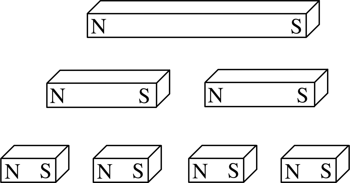
Figure 3 Cutting a bar magnet creates smaller bar magnets. It does not isolate individual north and south magnetic poles.
The concept of a magnetic pole is of great value in qualitative discussions of magnetic forces, but it is not particularly useful in quantitative work. The limitation arises from the fact that in practice it appears to be impossible to isolate either a north magnetic pole or a south magnetic pole. If, for instance, you cut a bar magnet in half, instead of obtaining two separate magnetic poles you will simply produce two small bar magnets, each with a north pole and a south pole (see Figure 3).
This continues to be the case no matter how finely you subdivide the original magnet. Even individual atoms or atomic constituents such as electrons and protons are magnetically similar to tiny bar magnets, not to isolated magnetic poles. Our inability to completely separate north and south poles contrasts sharply with the relative simplicity of separating positive and negative electric charges and means that magnetic phenomena have to be treated somewhat differently from the electrical phenomena with which they otherwise have a great deal in common.
Before leaving the subject of magnetic poles its worth noting one further point, even though it relates to matters far beyond the scope of FLAP. At the present time many of the theories which aim to describe the nature of the fundamental constituents of all forms of matter, i.e. the ‘elementary particles’ of nature, do predict the existence of particles that have the magnetic properties of isolated poles. These hypothetical particles are referred to as magnetic monopoles. Such monopoles have never been convincingly detected, despite one or two claims to the contrary, and it is widely believed that even if they do exist they are so rare that they are never likely to be observed. i However, if magnetic monopoles do exist they are expected to exert forces on one another similar to those between isolated electric charges. In particular, if two stationary magnetic monopoles are separated by a distance r then the force that each experiences due to the other will have a magnitude given by
F = C/r2
where C is a constant. This formula shows that the magnetic force between monopoles is expected to satisfy an inverse square law just like the electrostatic force between point charges. i Our inability to separate magnetic poles and to produce monopoles means that this formula is actually of much less use in the description of physical phenomena than its electrical counterpart (Coulomb’s law). It is this difference that accounts for a good deal of the mathematical complexity that arises in the description of magnetism.
2.3 Magnetic fields
The fact that magnets interact even when at a distance from one another is usually explained in terms of a magnetic field. The main purpose of this subsection is to introduce magnetic fields and to explain how they can be determined. You will also see how such fields can be represented mathematically and pictorially.
In physics the term field is generally used to denote a physical quantity to which a definite value may be ascribed at each point in some region of space at a given time. For example, the fact that a definite temperature can be associated with each point in the room you are now occupying means that there is a temperature field in the room. This is said to be a scalar field since its value at any point (at a particular time) is determined by a single scalar quantity – the temperature T at that point. We can denote this field by T (x, y, z) where the Cartesian coordinates x, y, z can be used to identify any point in the room, and serve to emphasize that the temperature generally varies with position. The quite separate observation that a particle of mass m located at any point with position coordinates (x, y, z) experiences a downward force, Fgrav due to gravity can be explained saying that there is a gravitational field throughout the room. The gravitational field at any point (x, y, z) is conventionally defined as the gravitational force per unit mass that would act on a ‘test’ mass i m at that point and is denoted by g (x, y, z), so we can write
${\bi g}(x,\,y,\,z) = \dfrac{{\bi F}_{\rm grav}\text{(on a mass }m\text{ at }(x,\,y,\,z))}{m}$
Note that in this case the field is specified by a vector at every point – a quantity with magnitude and direction – and is therefore said to be a vector field. Our use of a bold symbol (g) to represent the field indicates its vectorial nature. An electric field E (x, y, z) may be defined in much the same way, as the electrical force per unit charge that would act on a test charge placed at any point (x, y, z)
${\bi E}(x,\,y,\,z) = \dfrac{{\bi F}_{\rm el}\text{(on a charge }q\text{ at }(x,\,y,\,z))}{q}$
Now the magnetic field in some region of space must describe magnetic forces, so we might reasonably expect it be a vector field, just like the gravitational and electric fields. This is indeed the case and we usually denote the magnetic field at (x, y, z) by B (x, y, z). But in the absence of isolated magnetic poles (the magnetic equivalent of masses and charges) how are we to specify the magnitude and direction of this field?
Defining the direction of a magnetic field
It is relatively easy to define the direction of a magnetic field. There are a number of ways in which it might be done, but in view of what was said earlier the most obvious is to use a compass. We know that a compass needle tends to take on a specific alignment in the presence of a magnet, so we can define the direction of a magnetic field at any point as the direction indicated by the north pole of a compass needle placed at that point. This sounds like an eminently sensible way of defining the direction of a magnetic field, though we actually need to be think a little more about the details if we are to use it in a wide range of circumstances. For instance, if dealing with a magnetic field that changes direction over a small region of space (such as the magnetic field inside an electronic device) we would have to use a very tiny compass indeed, so we should really imagine that we are determining the direction with a vanishingly small compass that can effectively show us the direction of the field at a point. Moreover, we need to be aware that the magnetic field at a given location may point in any direction; it is not necessaily horizontal.
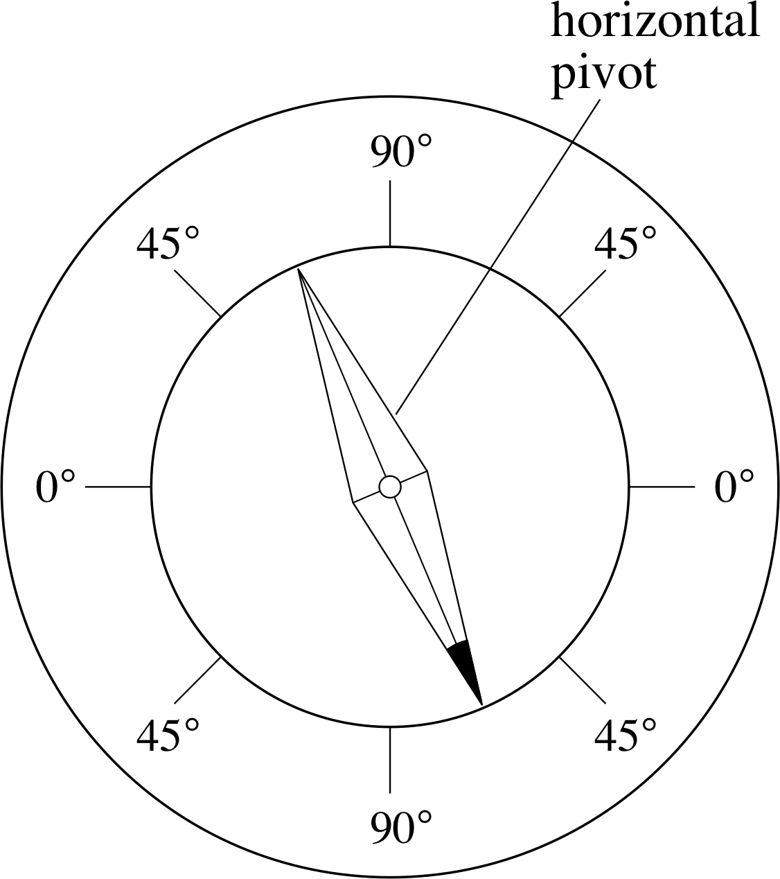
Figure 4 An inclinometer or dip circle, used for measuring the angle of the Earth’s field with respect to the horizontal.
Consequently, if we use a compass needle to define the direction of the field we must either make sure that the needle is free to rotate in three dimensions, or we must use two needles (one rotating horizontally and the other vertically) to determine the three–dimensional orientation at any point. When dealing with the magnetic field of the Earth it has been traditional for centuries to use two needles. The angle between the Earth’s magnetic field and the horizontal at any point is called the angle of inclination or the angle of dip and the device that uses a vertically rotating needle to measure that angle is called a dip circle or an inclinometer (Figure 4).
Of course, if you think that all this talk of vanishingly small compasses that are free to rotate in three dimensions is unnecessarily complicated you can just say that:
The direction of a magnetic field at any point is the direction of the magnetic force that would act on an isolated north magnetic pole (if we had one) placed at that point.
But you shouldn’t expect to determine the field direction by this method in practice.
Defining the magnitude of a magnetic field
Defining the magnitude B (x, y, z) = | B(x, y, z) |, of the magnetic field B (x, y, z) is a good deal more difficult than defining its direction. i Fortunately the intimate relationship between electricity and magnetism can aid us here. Once the direction of a magnetic field has been determined at some point, or better still in some small region, it is easy to place a wire at right angle to the field and to send an electric current through that wire. When this is done it is easy to show that the magnetic field exerts a force on the current carrying wire. The current in the wire is composed of moving charged particles, and the force that acts on the wire is one manifestation of the general observation that a magnetic field exerts a force on any moving charged particle, provided the particle is not travelling parallel to the field. The general relationship between the magnetic field B at a point, the velocity υ of an electrically charged particle as it passes through that point, and the magnetic force Fmag that acts on the particle is a little complicated so we will not discuss it here. We can say that in the special case when a particle of positive charge q passes through the point (x, y, z) with speed υ⊥ along a direction at right angles to the magnetic field at that point, it will be subjected to a force of magnitude
Fmag = qυ⊥B (x, y, z)
where B (x, y, z) is the magnitude of the magnetic field at the point (x, y, z).
Rearranging this equation (and providing a little more explanation) we can define the magnitude of the magnetic field at the point (x, y, z) by
$B(x, y, z) = \dfrac{F_{\rm mag} \text{(on }q\text{ as it moves through the point }(x, y, z))}{q\upsilon_{\perp}}$(1) i
Since the magnetic force magnitude Fmagmay be measured in newton (N), the charge q in coulomb (C) and the perpendicular speed υ⊥ in metres per second (m s−1), it follows that the magnetic field strength can be measured in units of N s C−1 m−1. This is a sufficiently important combination of units that it is given its own SI name and symbol.
The SI unit of magnetic field strength is the tesla (T), where 1 T = 1 N s C−1 m−1 i
It is worth noting that the tesla is large unit by everyday standards. The magnitude of the Earth’s magnetic field over much of its surface is around 10−5 T, and a typical bar magnet might produce a field of magnitude 10−2 T within a centimetre or two of its pole pieces.
✦ A proton (charge e = 1.60 × 10⁻¹⁹ C) travels with speed 4.00 × 10⁶ m s−1 through a point at which there is an intense magnetic field of magnitude 2.50 T. Assuming that the proton is moving at right angles to the field at the point in question, what is the magnitude of the instantaneous magnetic force on the proton?
✧ Using Fmag = qυ⊥B, in this case
Fmag = 1.60 × 10−19 C × 4.00 × 106 m s−1 × 2.50
i.e.Fmag = 1.60 × 10⁻¹² N
Representing a magnetic field
Figure 2 The Earth’s magnetic and geographic poles and the Earth’s magnetic field.
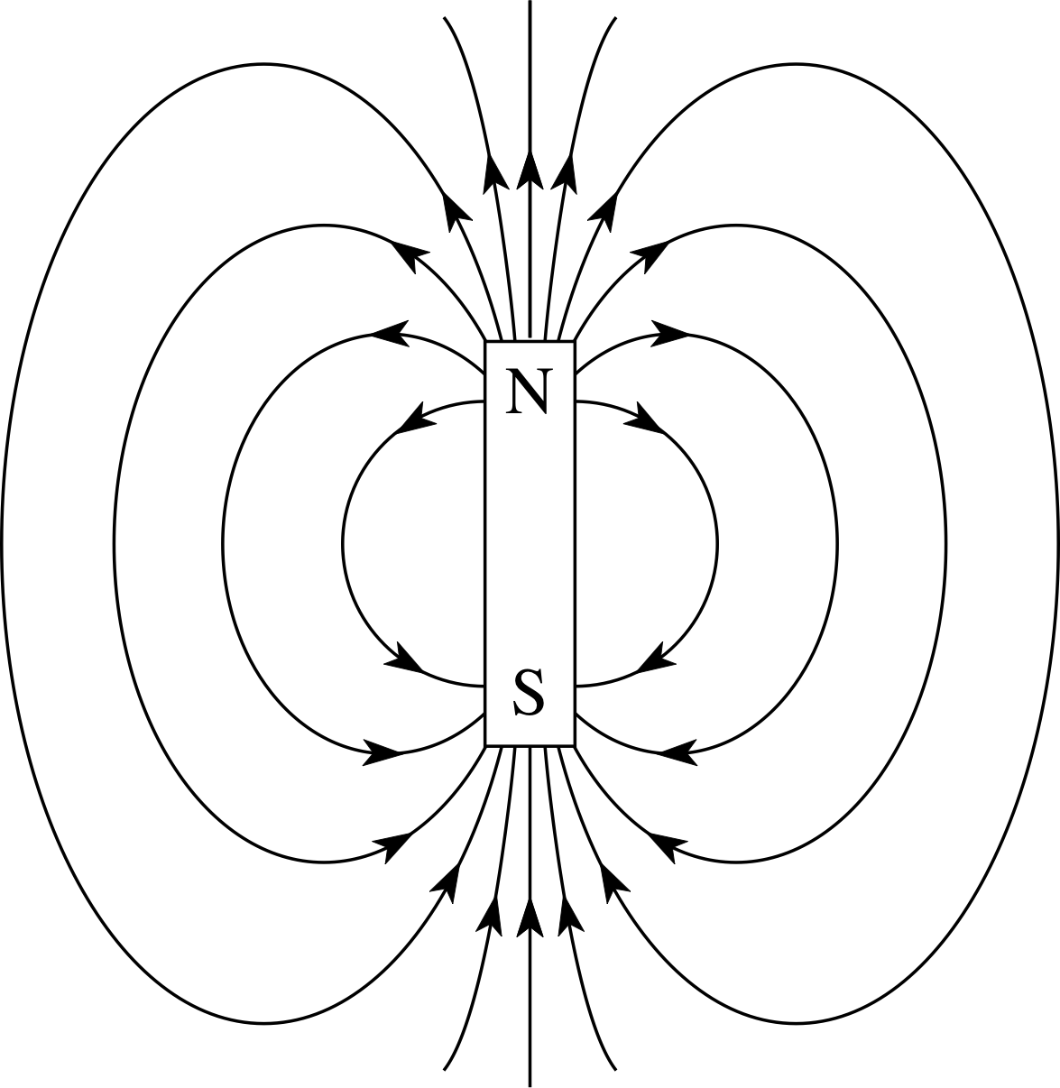
Figure 5 The magnetic field of an isolated bar magnet represented (approximately) by magnetic field lines.
It is often necessary to represent magnetic fields on diagrams. This may be done by using magnetic field lines. These are directed lines (i.e. lines with arrows on them) that have the following properties:
- The lines are drawn so that at any point the magnetic field is tangential to the lines. i
- The direction of the field line at any point indicates the direction of the magnetic field at that point (i.e. the direction that the north pole of a compass would point, or an isolated north pole would tend to move).
- The density of the field lines in any region is proportional to the magnitude of the magnetic field in that region.
In practice the last of these conditions is quite hard to satisfy, especially if you are trying to represent a three–dimensional field (such as that of the Earth) on a flat piece of paper (as in Figure 2). For that reason most field line representations of magnetic fields are at best approximate.
With this in mind, look at Figure 5 which shows the magnetic field of a bar magnet. Since the bar magnet essentially consists of two opposite magnetic poles of equal strength separated by a fixed distance it is sometimes described as a magnetic dipole, and the field that it produces is said to be a dipolar field. Figure 5 makes no attempt to show the three–dimensional nature of the field; it is restricted to the plane of the page. Furthermore it is only an approximate representation of the field; the field lines near the mid–point of the magnet have been drawn with roughly equal separations, indicating that the field is of uniform magnitude in that region whereas in reality the magnitude of the field would actually decrease as the distance from the magnet increased. Nonetheless, the diagram gives a clear (and correct) impression that the field of the dipole is the vector sum of the fields from the poles at either end of the magnet.
In plotting the field of a magnet, as in Figure 5, we would not normally attempt to nullify the Earth’s field. The observed field would therefore be the resultant vector sum of the fields of the Earth and the magnet. However, provided we restrict the plot to points close to the magnet, where the magnet’s field is much larger than the Earth’s field, then it would be a fairly accurate representation of the magnet’s field.
✦ As we plot the field at points which are further away from the magnet, what happens to the relative magnitudes of the fields of the Earth and of the magnet?
✧ The strength of the magnet’s field diminishes as we get further away from it, and eventually it will become much less than the Earth’s field, which is constant over such a small region, and so will then dominate. At intermediate distances the Earth’s field and the magnet’s field will be comparable in size.
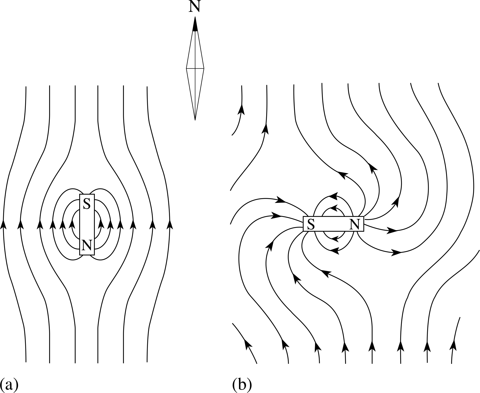
Figure 6 Field plot of a bar magnet with N–pole pointing (a) south and (b) east.
Just how the bar magnet’s field and the Earth’s field merge will depend on the orientation of the magnet. Figures 6a and 6b show extended plots when the magnet has its N–pole pointing south and east, respectively. Note that there are regions where the fields of the Earth and the magnet are almost equal and opposite, so the resultant field is very weak and the field lines correspondingly far apart.
There is one further important feature of field line plots: field lines will never be found to cross each other because that would imply that a compass placed at the cross–over point would have to point in two directions at once! i
Another method of finding the shape of the field pattern near a magnet is to cover the magnet with a horizontal sheet of paper and to sprinkle fine iron filings evenly over the paper. i When the paper is tapped gently, the filings tend to congregate in the regions of high field and also to show some line structure in the pattern. This similarity between the lines of filings and field line patterns can be very misleading as it may be interpreted as meaning that the magnetic field exists only along these lines, and that at points in between the lines there is no field. In fact, using a compass, we can follow a field line anywhere we like in the vicinity of a magnet (provided our starting point is not one at which the the field is zero) because the field is continuous from point to point. The apparently significant lines of filings are quite fortuitous and arise through the existence of a few, perhaps larger, filings which are more reluctant to move when the paper is tapped, and so provide a centre to which other filings are attracted.
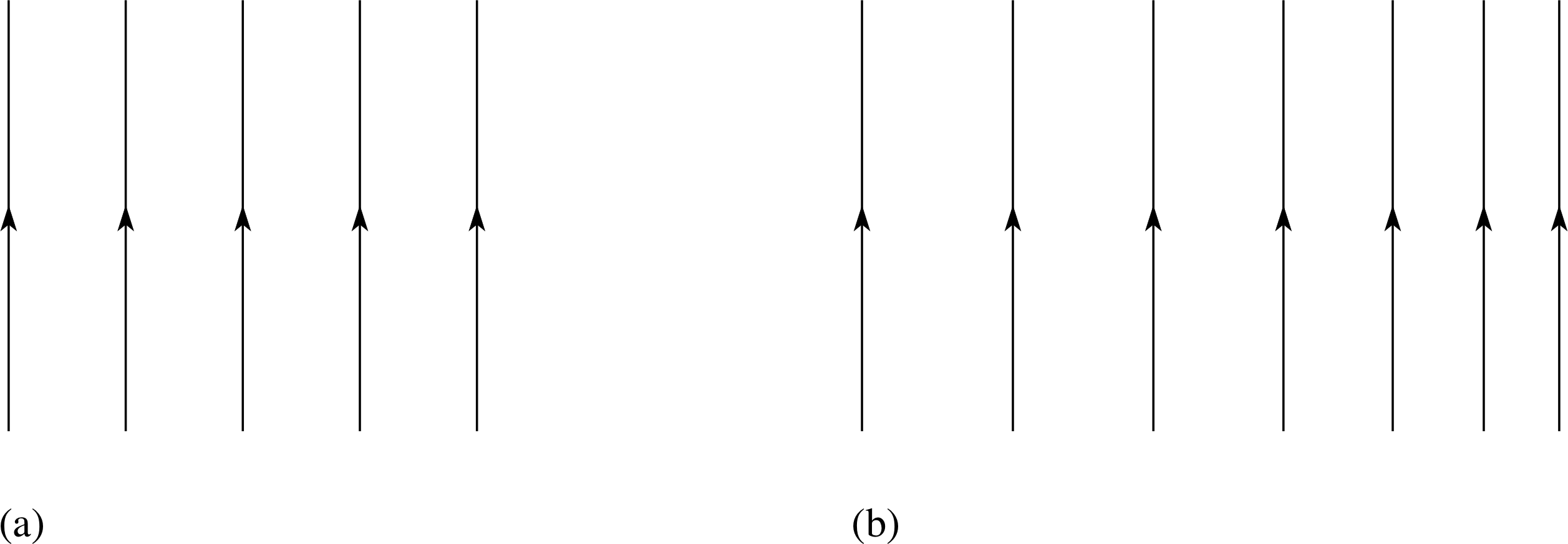
Figure 7 Examples of different magnetic fields.
✦ (a) If Figures 7a and 7b represent the magnetic field lines in some region of space, describe the corresponding magnetic fields.
(b) If Figures 7a and 7b represent patterns of iron filings, rather than field lines, what can you now say about the magnetic field.
✧ (a) The uniform spacing of the field lines in Figure 7a indicates that the magnetic field itself is uniform in this region, i.e. it has the same magnitude throughout the region. The direction of the field is the same at every point, and is everywhere parallel to the field lines. In Figure 7b, the greater density of field lines at the right of the diagram indicates that the magnitude of the field is greater there.
(b) If the lines in Figures 7a and 7b represent patterns of iron filings their density does not necessarily indicate the relative strength of the field in the different parts of the region. (Nor would the arrows have any obvious significance.)
Question T1
Sketch the magnetic field plots for a bar magnet in the Earth’s field with its N–pole pointing (a) north, and (b) west. i
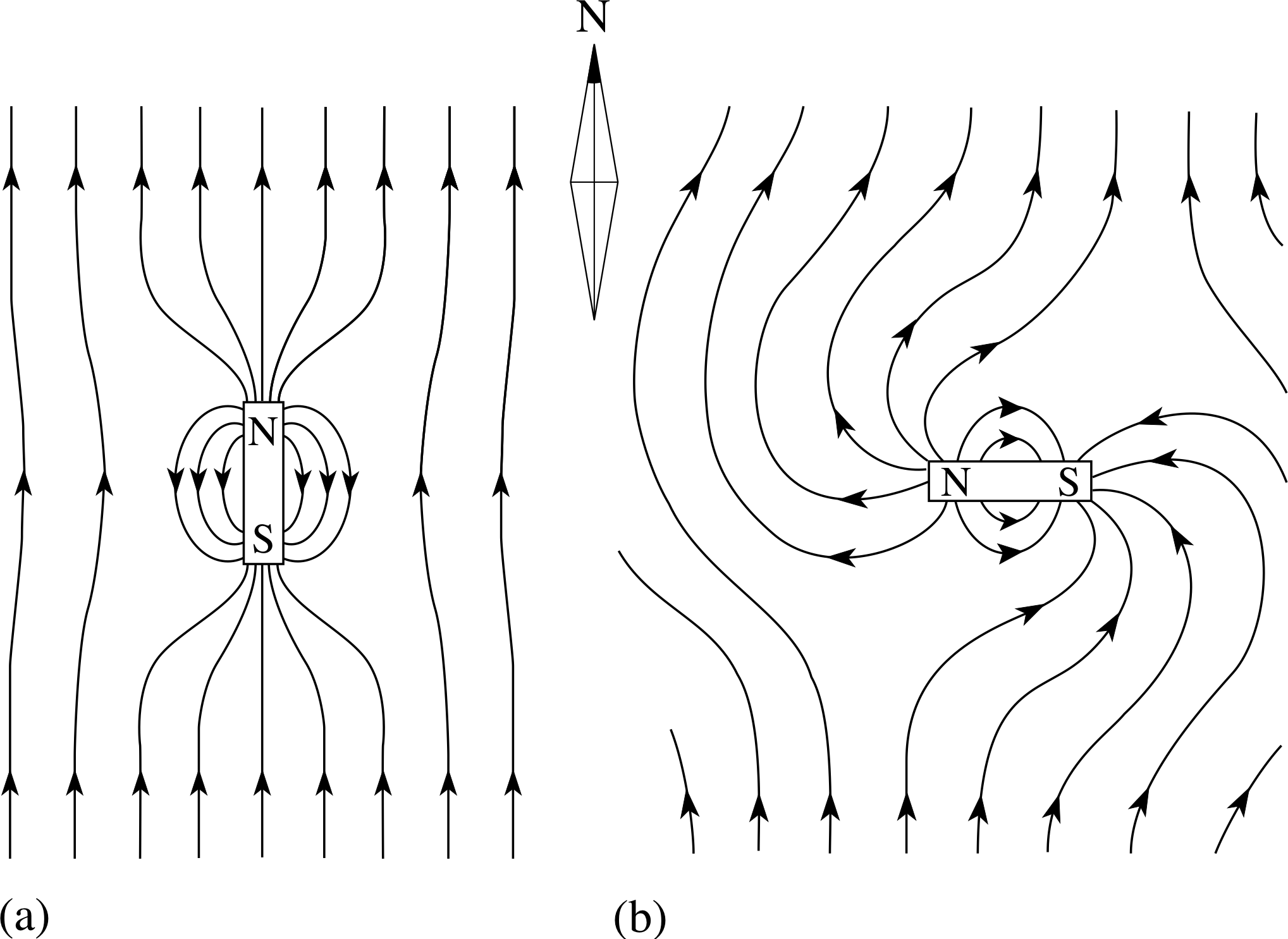
Figure 25 See Question T2.
Answer T1
Field plots for a bar magnet in the Earth’s field: with north pole pointing (a) north, and (b) west are shown in Figure 25.
We can think of the field lines as if they were fastened to the magnet in the region of the poles, so that when the magnet is rotated from position (a) to position (b), it appears that the field lines are pulled around with it.
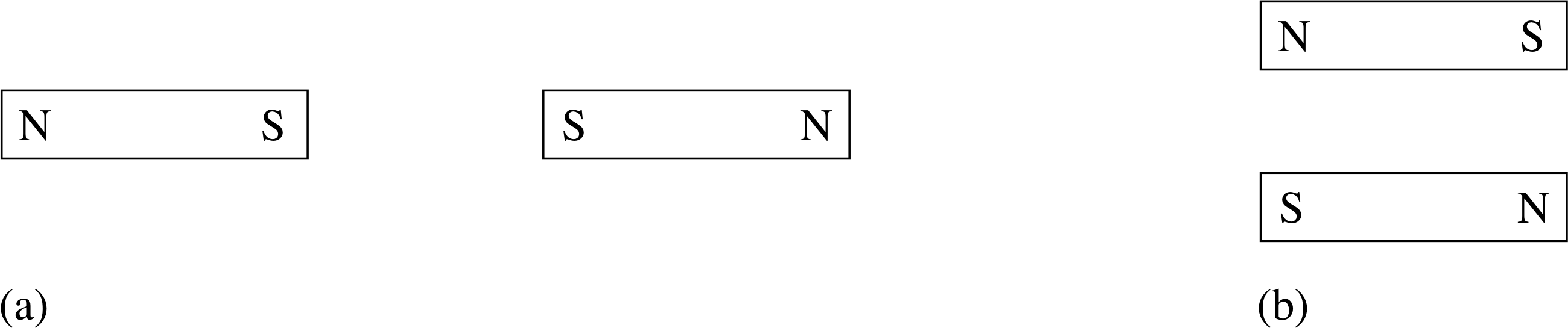
Figure 8 See Question T2.
Question T2
Sketch magnetic field plots for the magnets shown in Figure 8. (Assume that the Earth’s contribution can be ignored.) i
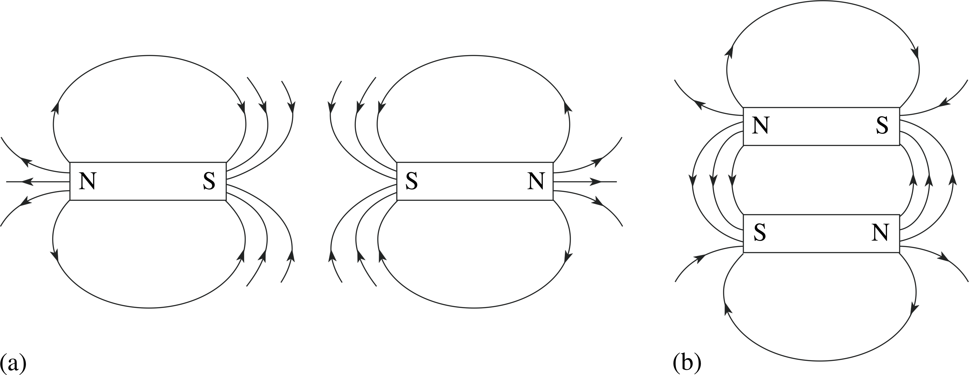
Figure 26 See Question T2.
Answer T2
The field plots are shown in Figure 26. (If possible you could also check the results using two bar magnets and iron filings or a small compass.)
2.4 Magnetic materials
As was described earlier, a very simple test of the magnetic properties of different materials is to see if they are attracted by a magnet. This test provides an easy and immediate classification into materials which are strongly attracted and those which are not. The former group has been found to consist primarily of five elements – iron (Fe), cobalt (Co), nickel (Ni), gadolinium (Gd) and dysprosium (Dy) i – and some associated alloys. i These are known as ferromagnetic materials, taking their name from iron, the most common member of the group. Materials which are apparently unaffected by a magnet do in fact have weak magnetic properties, some are actually repelled by a magnet, but such effects are seen only with very sensitive apparatus and we will not discuss them further.
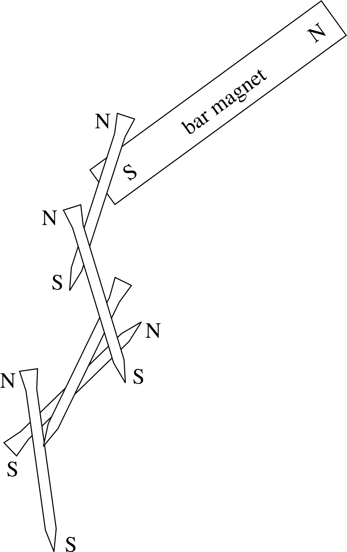
Figure 9 Magnetic induction enables a magnet to lift a chain of nails.
If we place a bar magnet near to a rod of pure iron, then the rod and the magnet are attracted to one another. When, however, the bar magnet is removed, the iron retains (almost) none of its magnetic properties. We say that these magnetic properties are induced in the iron rod by the bar magnet, that is to say that the magnet’s field causes the rod to change temporarily into a magnet. Further observation shows that the force between the magnet and the rod is always one of attraction, from which we deduce that the induced pole at the near end of the rod is always of the opposite polarity to the adjacent end of the magnet. This process of magnetic induction can be extended. If we put the rod in contact with the magnet, it acts like an extension of the magnet and it, in turn, can attract a further rod and so on, but with the strength of the attractive forces becoming weaker, as we go further from the magnet. This is a familiar result – a permanent magnet can lift a chain of nails or pins (Figure 9), but when the magnet is forcibly removed from the first nail or pin, the rest fall. The induced magnetism is only temporary, and disappears when the inducing field is removed.
Materials, such as pure iron, which depend (almost entirely) on the presence of another magnet for their magnetism are described as magnetically soft. In contrast, steels are examples of alloys made by adding other elements (typically carbon) to iron. These materials are harder to magnetize, but once they are magnetized they do not easily become demagnetized. Such materials are said to be magnetically hard and are the materials from which permanent magnets are made. The study of permanent magnetism is an area of great technological importance, but one with unexpected results. For example, the simple addition of small amounts of copper (a non–ferromagnetic material) to carbon steel produces magnets of much greater strength.
Another group of magnetic materials, known as ferrites, are brittle ceramics made by sintering oxides i of iron and barium (Ba). Granules of these ceramics can also be bonded with plastics or rubber to give flexible magnets (such as refrigerator seals) and are also used to make magnetic audio and video tapes, or floppy disks for computers. Information is recorded on tapes or disks by magnetizing their ferromagnetic grains through the application of a localized external magnetic field that is generated by, and is proportional to the strength of, the signal being recorded. The stored information can be erased with a strong magnetic field, allowing the tape or disk to be reused.
Scientific studies of the magnetic properties of materials are far more sophisticated than this brief discussion might indicate. Research into the magnetic properties of materials has been, and continues to be, one of the most active areas of physics. International conferences entirely devoted to magnetism are held on a regular basis and there is a very large annual output of books and scientific papers dealing with magnetic materials.
With the understanding of atomic structure and quantum mechanics has come an appreciation that ferromagnetism and permanent magnetism have their origins almost entirely in the intrinsic properties of the electrons (electron spin magnetism) which make up their constituent atoms. i
Question T3
Should the materials used in the storage of information be magnetically soft or magnetically hard?
Answer T3
The materials should be magnetically hard so that they retain the information in the absence of the magnetic field used to record it.
3 Magnetic fields produced by electric currents: electromagnetism
3.1 Introduction to electromagnetism
In 1820, a Danish philosopher and scientist, Hans Christian Oersted, performed the first experiment to show an interaction between an electric current and a compass needle. This association of magnetic fields and currents provided the basis for a new branch of physical science – electromagnetism. Electromagnetism is a major topic within physics and in this module we are able only to give the briefest of introductions to it. i
Oersted showed that a current in a wire could, in certain circumstances, cause the deflection of a compass needle placed nearby. The greatest deflection was produced with the wire in a horizontal plane parallel to the undeflected needle and either above or below it. Oersted also found the important result that reversing the current reversed the direction of the deflection. Subsequent experiments soon extended Oersted’s results. For example, as you will see later in this section, the field of a bar magnet can be reproduced using current in a coil. i Although permanent magnetism was discovered before electromagnetism, permanent magnetism could not be understood until quantum mechanics arrived and it was the understanding of electromagnetism which allowed progress in classical physics to be made, culminating in an understanding of light as an electromagnetic phenomenon. We will follow the early stages of this course of development in this module.
3.2 The magnetic field of a long straight current
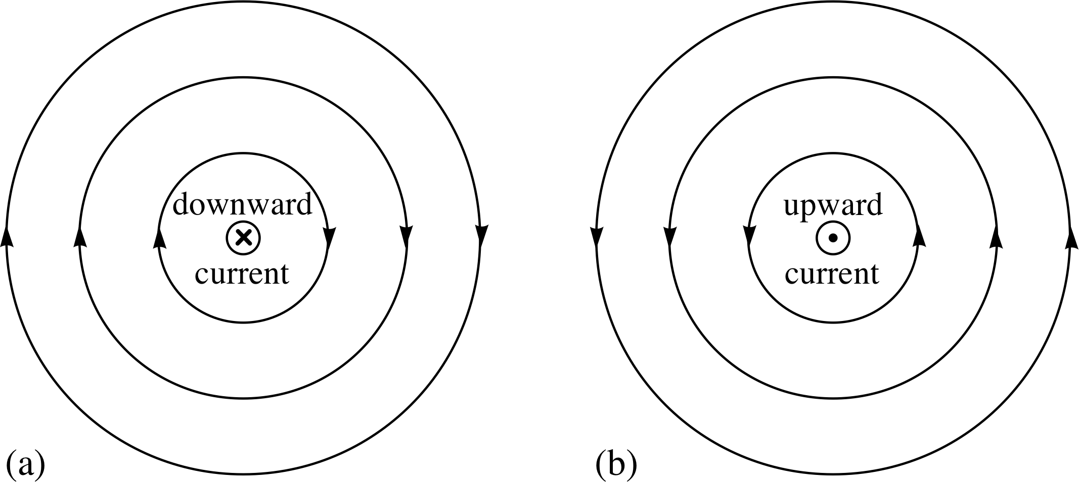
Figure 10 Circular magnetic field lines produced by a current in a long straight wire with the current pointing (a) downwards, and (b) upwards. i
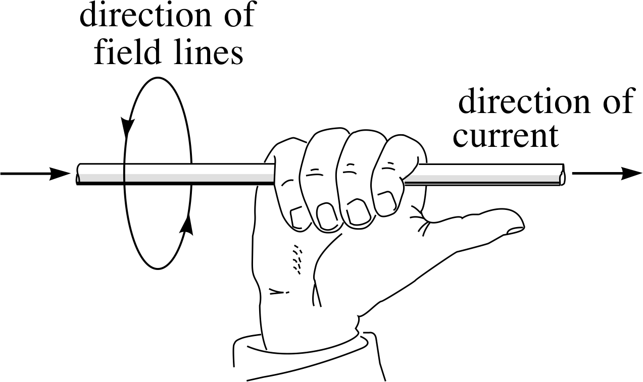
Figure 11 The right–hand grip rule. The fingers curl about the pointing thumb in the same sense as the field lines curl about the current.
A further simple experiment leads to an explanation of Oersted’s results. If you pass a vertical current carrying wire through a horizontal card on which you place a compass, then you can plot the magnetic field produced by the current. The field lines are found to be closed loops about the wire. With a sufficiently large current these loops are circles concentric with the wire, as shown in Figure 10. i
Iron filings may also be used to show the field pattern, but this needs currents of some tens of amps (or several adjacent wires, each carrying more moderate currents in the same direction).
The direction of the field lines depends on the direction of the current. If the direction of current is reversed, then the direction of the field lines is also reversed, as is shown in Figure 10.
Fortunately, there is an easy way to remember the field directions. Just close the palm of your right hand with thumb extended and point your thumb in the direction of the current shown in either diagram of Figure 10.
In each case you will find that your fingers curl around your thumb in exactly the same way that the magnetic field lines curl around the current. This simple way of remembering the direction of the magnetic field is illustrated in Figure 11 and is known as the right–hand grip rule.
We can now use the right–hand grip rule to explain why Oersted obtained a compass deflection in some positions relative to the wire and not in others.
✦ In which of the following situations will there be a deflection of the compass?
(a) When the undeflected compass lies in a horizontal plane, directly above or below the horizontal wire, with the compass needle initially pointing parallel to the wire.
(b) When the undeflected compass is initially pointing towards the wire, in the horizontal plane containing the wire.
✧ The magnetic field lines produced by a current in a long straight wire circulate about the wire. So, in (a) there will be oppositely directed horizontal forces on the two ends of the compass needle which will in general cause a deflection (Figure 12a), with the compass needle adopting the direction of the resultant of the current’s field and the Earth’s field.
For the situation described in (b), where the wire is horizontal, then to the sides of the wire the field will be directed vertically upwards or downwards: a normal compass needle, being designed to rotate in the horizontal plane, cannot respond to such a vertical field. Therefore in (b) there will be no deflection (Figure 12b).
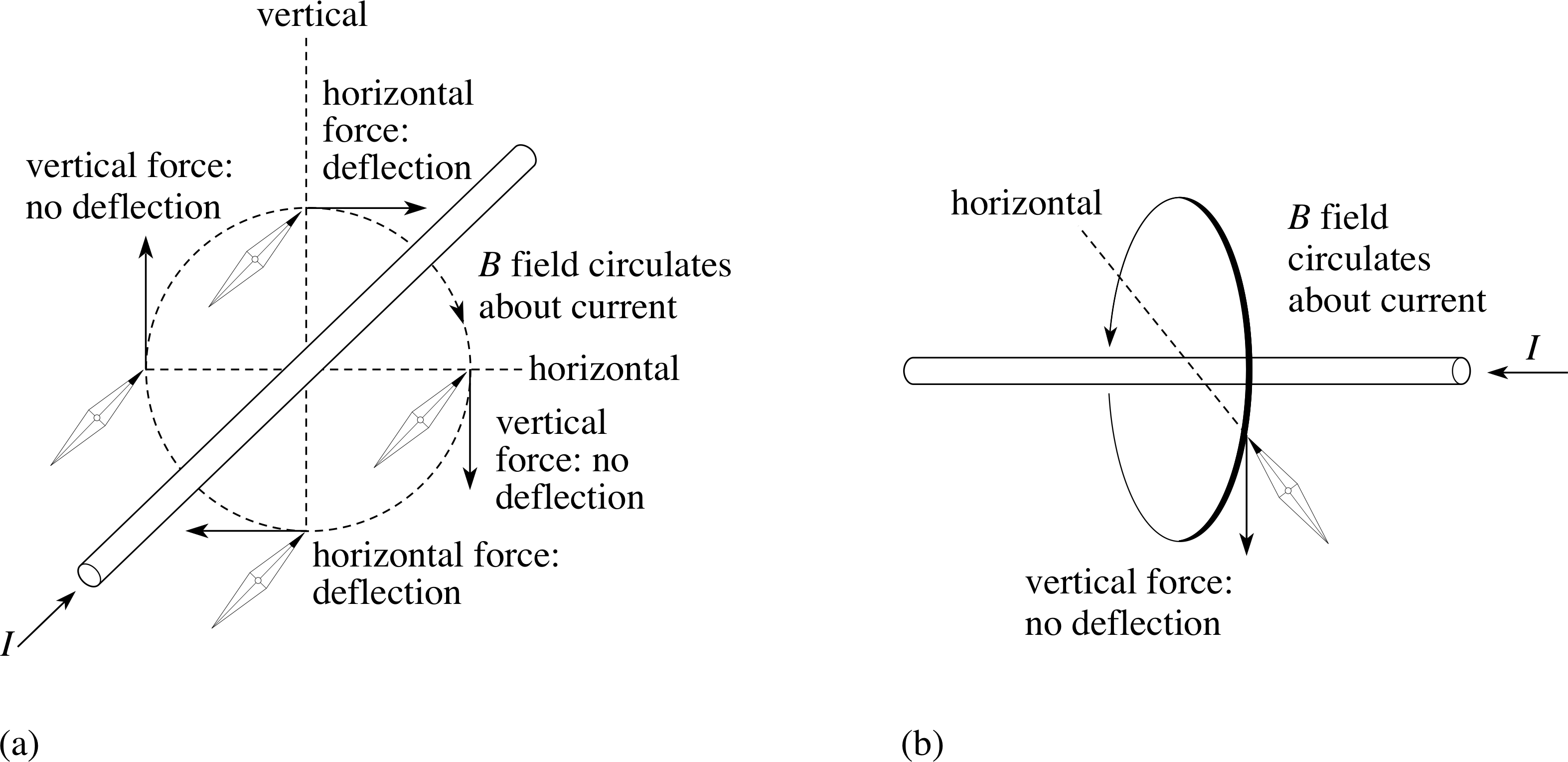
Figure 12 (a) Here the wire is in the horizontal plane and the current is S to N. The field it produces at the sides is vertical and the compass cannot respond but the field above and below is horizontal and the compass will be deflected, either to the W or to the E.
(b) With the current from W to E, the compass to one side of the wire experiences a vertical force and cannot respond. A compass placed below the wire has an additional force aligning it N–S.
As well as its direction, we generally also want to know the strength of a magnetic field. At a perpendicular radial distance r from a long straight wire, the magnitude of the magnetic field vector (or the magnetic field strength), for which we use the symbol B (r), is proportional to the current I in the wire and inversely proportional to the distance r. i This relationship is normally expressed as:
Magnetic field strength at a distance r from a long straight wire is:
$B(r) = \dfrac{\mu_0I}{2\pi r}$(2)
where μ0 (pronounced mew-nought) is a constant, called the permeability of free space, I is the current and r is the perpendicular distance of the point from the wire.
First, notice that the form of Equation 2 is physically reasonable. It shows that if the current is increased, so is the strength of the field that it produces at a fixed distance from the wire. Also, for a given current, the field gets weaker as the distance from the wire increases. Equation 2 has a very simple form because the field produced by this current is highly symmetrical – the field strength at any point is determined by the perpendicular distance from the wire.
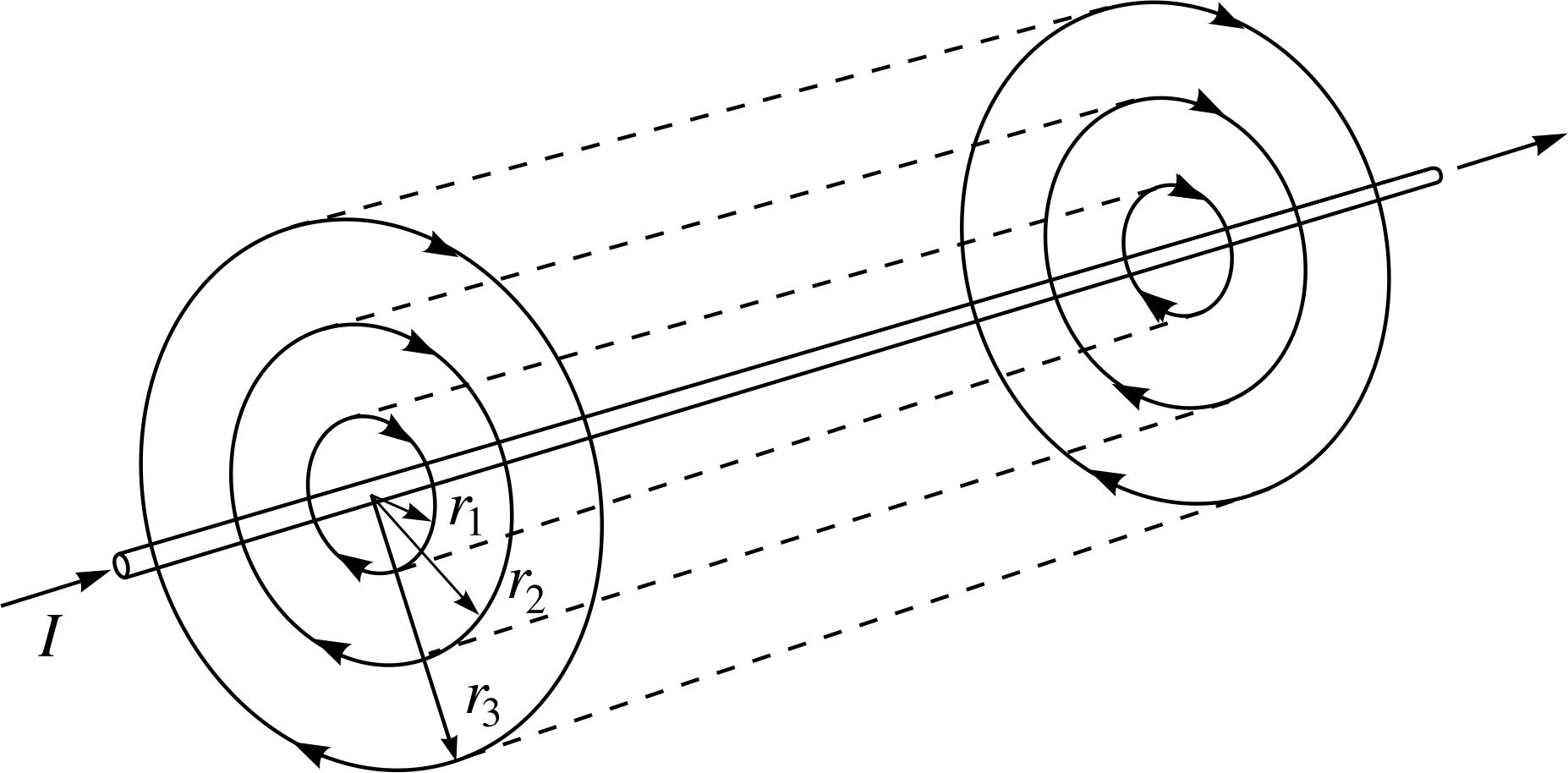
Figure 13 The field strength is the same at any point on the surface of a cylinder which is coaxial with the wire. It is different for each cylinder.
If you imagine a set of coaxial cylinders drawn around the wire, as shown in Figure 13, the field strength is the same at all points on the surface of any one cylinder, but is different for each cylinder.
Second, notice that Equation 2 is not a vector equation – it shows the magnitude of the field but not its direction. A magnetic field is a vector field and we could write a more complicated vector equation which would fully describe both its magnitude and direction. We will, instead, rely on the right–hand grip rule to tell us the field direction in this simple situation.
As noted earlier, the SI unit of the field strength B (r) is the tesla (abbreviated to T) and the SI unit of current is the ampere (A). With distances in metres Equation 2 then establishes the dimensions of the constant μ0 as T m A−1. i
The ampere itself is defined in terms of the force between two current carrying conductors and when this force is expressed in newtons, the numerical value for μ0 in SI units is fixed (i.e. no measurement of it is required) at μ0 = 4π × 10−7 T m A−1. Thus the choice of the name for μ0 is unfortunate, since μ0 does not describe some property of free space (i.e. of a vacuum) but is simply a constant which is defined to allow SI units to be used consistently in the equations.
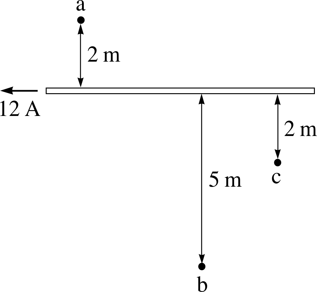
Figure 14 See Question T4.
Question T4
Figure 14 shows three points close to a wire carrying a current of 12 A. For each of the points a, b and c, calculate the local magnetic field strength, and state whether the magnetic field points into or out of the plane of the paper.
Answer T4
At point a, the magnitude of the field according to Equation 2,
$B(r) = \dfrac{\mu_0I}{2\pi r}$(Eqn 2)
is$B = \dfrac{4\pi\times10^{-7}\,{\rm T\,m\,A^{-1}\times 12\,A}}{2\pi\times2\,{\rm m}} = 1.2\times 10^{-6}\,{\rm T} = 1.2\,\mu{\rm T}$
Using the right–hand grip rule, the field points into the page at point a. Similarly, at point c, the field strength is B = 1.2 × 10⁻⁶ T and the field points out of the page. At point b (with r = 5 m) the field strength is B = 4.8 × 10⁻⁷ T and the field points out of the page.
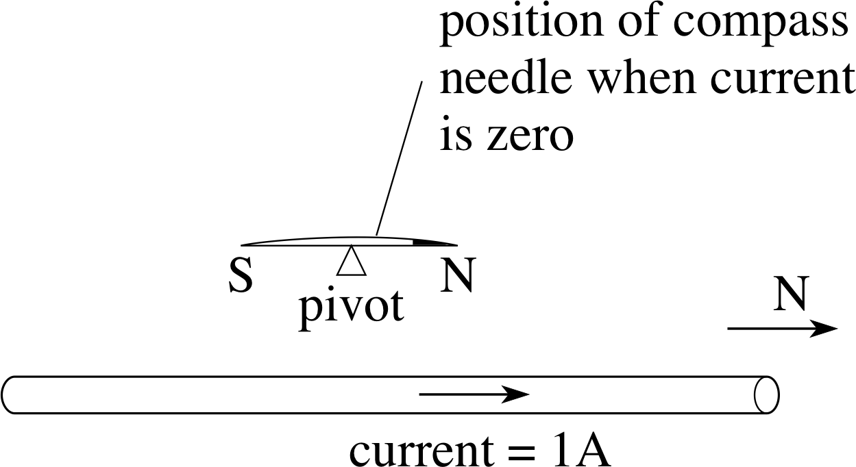
Figure 15 See Question T5.
Question T5
A horizontal straight wire carries a current of 1 A. At what distance is the magnetic field strength equal to that of the horizontal component of the Earth’s field (i.e. 20 μT). i If a compass is placed at this distance above the wire, in the arrangement shown in Figure 15, through what angle will the compass needle rotate?
Answer T5
Rearranging Equation 2,
$B(r) = \dfrac{\mu_0I}{2\pi r}$(Eqn 2)
and substituting B = 20 × 10−6 T, we find
$r = \dfrac{\mu_0I}{2\pi B} = \dfrac{4\pi\times 10^{-7}\,{\rm T\,m\,A^{-1}\times 1 A}}{2\pi\times 20\times 10^{-6}\,{\rm T}} = 1 \times 10^{-2}\,{\rm m}$
The current’s field and the Earth’s field are mutually at right angles and (at this position) they have equal strength, so the resultant is at 45° to both and that is the angle through which the compass will rotate.
Finally, we note one further point concerning the magnetic fields produced by current in straight wires. If we have a bundle of straight wires, all close together and each carrying a current in the same direction, then the total magnetic field produced at some point by the bundle will be the vector sum of the fields produced by the individual currents. This is an example of the principle of superposition – which is an extension of a familiar result concerning forces. If several forces act on a body at the same time, then the resultant force is the vector sum of those forces taken one at a time. If the forces are produced by the magnetic fields of several different currents, then the resultant force can be found by adding the forces due to the separate currents – in other words, the resultant magnetic field is the vector sum of the individual magnetic fields due to the separate currents.
For a bundle of wires each carrying a current, the resultant field will be approximately the same as if we had the same total current flowing in a single wire. We say ‘approximately’ because the wires in the bundle will not all be in precisely the same position as the single wire: the larger the distance from the bundle, the more accurate this approximation will be.
3.3 The magnetic field of a current in a circular loop

Figure 16a Magnetic field components produced by small elements of a circular loop of wire.
If we know the shape of the magnetic field due to a long straight wire carrying a steady current, it is fairly easy to build up pictures of the sort of magnetic fields that are produced by other configurations of current carrying wires.
Imagine taking a long straight wire and bending it into a circle. At any particular point on the wire, the field lines will be concentric circles about the wire, at least to the extent that the influence of other parts of the wire can be ignored, as shown in Figure 16a. Of course, in the real world, the points on the wire cannot be considered in complete isolation and the pattern of field lines sketched in Figure 16a is therefore only an approximation.

Figure 16b An accurate representation of a cross section of the field through a circular loop; the full field pattern comes from the rotation of the figure around the vertical axis of symmetry of the loop.
To obtain a more accurate result, it is necessary to add vectorially all the small magnetic field components created by the various small sections of the wire. The mathematics of such a sum is beyond the scope of this module, but the rough shape of the field pattern is clear from Figure 16b. For example, in the centre of the loop the fields due to each individual part of the wire reinforce one another, with all the field lines pointing downwards through the middle of the loop.
When the vector addition of all the field contributions is performed to give the total field strength, then the magnetic field strength at the centre of the loop is found to be given by:
Magnetic field strength at the centre of a circular loop is:
$B_{\rm loop}= \dfrac{\mu_0I}{2R}$(3)
where I is the current and R is the radius of the loop.
Even without deriving this equation it is easy to see that its form is physically plausible: the larger the current, the stronger the magnetic field that results. Also, for a given current, the bigger the loop (i.e. the further away the centre is from the wire), the weaker the field will be at the centre of the loop.
✦ Check that the units on the right–hand side of Equation 3 do reduce to tesla.
✧ The units are those of μ0 × I/R, i.e. T m A−1 × A × m−1 = T.
Question T6
The wire in Figure 16b consists of a single loop. How would you expect the field pattern and the strength of the field at the centre to change if the single loop were replaced by a compact coil of N turns, all having the same radius as the single turn? State any assumptions you make.
Answer T6
The word ‘compact’ implies that the turns of the coil are close together. At some distance away from the wires it would be difficult to distinguish between N turns of wire each carrying a current I and one turn carrying a current NI. We would therefore expect the magnetic field strength at the centre of the coil to be given by
$B_{\rm coil} = \dfrac{\mu_0NI}{2R}$
provided that the distance between the turns of wire is very small compared with R.
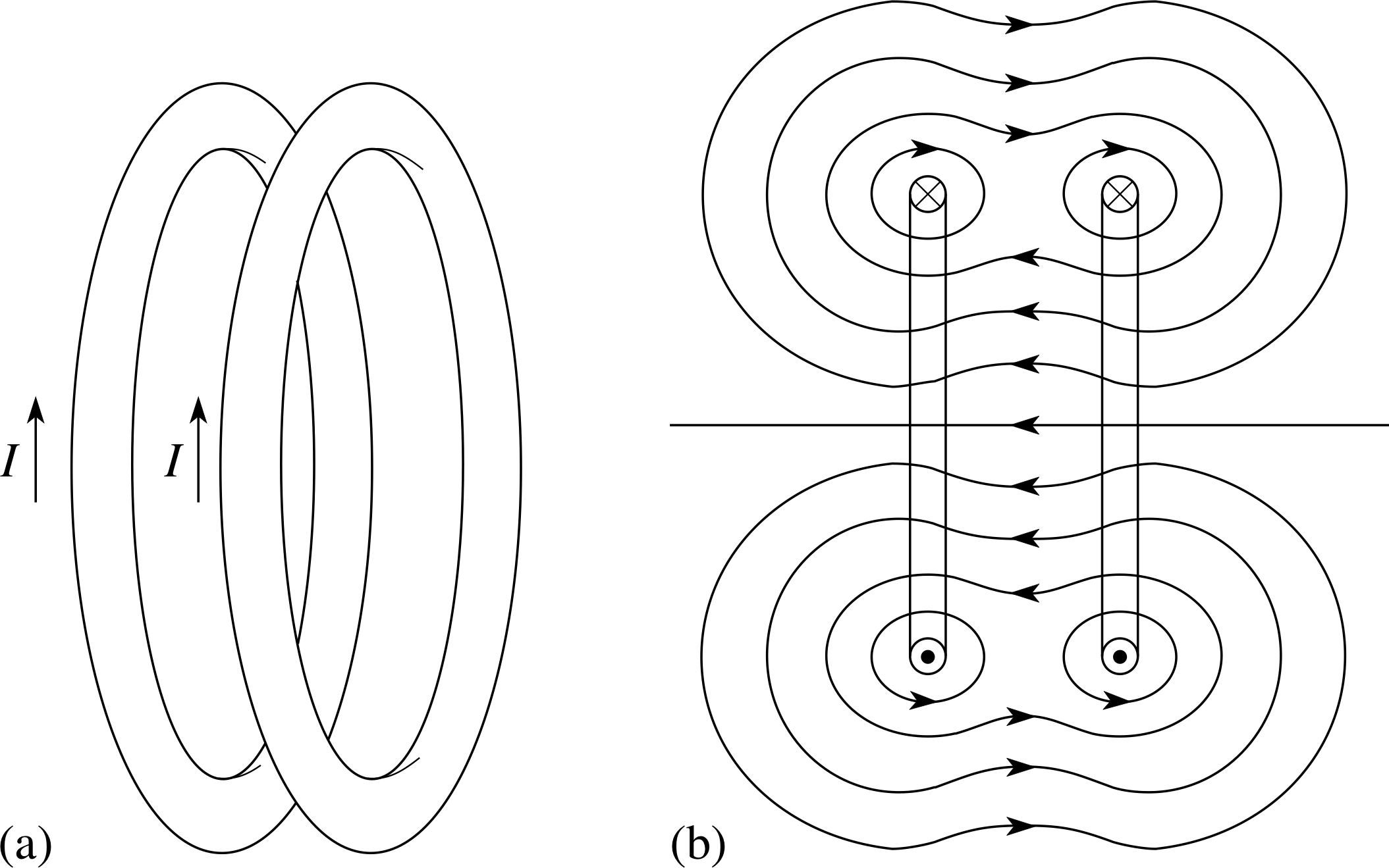
Figure 17 (a) Two similar circular current loops. (b) Bringing the loops together produces an extended region of uniform central field.
3.4 The magnetic field of a solenoid
Suppose we take a single loop of wire (as in Figure 16b), and place a second loop parallel to the first and a short distance away, as in Figure 17a. If the currents in the two loops circulate in the same sense, as shown, then the two loops produce similar fields at their centres. The fields are in the same direction and combine in the region of their centres to produce a continuous field, as in Figure 17b.
We now extend our two loops of wire into a whole series of loops, arranged sequentially and pushed close together. If each loop is connected to the adjacent loops, so that they form a single continuous coil, as illustrated in Figure 18a, then the coil so formed is called a solenoid and its shape is that of a helix.

Figure 18a A solenoid.
The resulting pattern of field lines is shown in Figure 18b for a loosely wound solenoid and in Figure 18c for a tightly wound solenoid.

Figure 18c (a) A solenoid. (b) The field from a loosely wound solenoid. (c) The field from a tightly wound solenoid.

Figure 18b The field from a loosely wound solenoid.
✦ Where else in this module have you previously seen a field like that shown in Figure 18c?
✧ Comparison with Figure 5 shows that the field of a bar magnet has the same shape as that of a solenoid.
Figure 5 The magnetic field of an isolated bar magnet represented (approximately) by magnetic field lines.
Calculations which are beyond the range of this discussion show that the magnetic field at any point inside an infinitely long solenoid is directed parallel to the axis of the solenoid and has a strength given by:
Magnetic field strength at any point within an infinitely long solenoid is:
$B_{\rm solenoid}= \dfrac{\mu_0NI}{L}$(4)
where N is the number of turns in a length L of the solenoid.
Question T7
(a) How would you interpret the quantity (N/L) in Equation 4?
(b) Suggest why we have said that Equation 4 applies to an infinitely long solenoid.
(c) No real solenoid can be infinitely long, so how might this situation be approximated in practical situations?
(d) Is the form of Equation 4 physically reasonable?
Answer T7
(a) N/L is the number of turns per unit length (so the magnetic field strength within the solenoid increases as the turns are packed closer together).
(b) As can be seen from Figure 18c, the field lines diverge towards the ends of the solenoid, showing that the field gets weaker there. In the case of an infinitely long solenoid, the field strength is the same at all internal points.
(c) The nearest we can get to a solenoid of infinite length, is a very long solenoid, where very long means having a length much greater than the diameter.
(d) We would expect the field to increase if the current is increased, and having more turns to the solenoid increases the number of contributions to the field at any point, so we would expect the field to increase with NI. We would also expect the field at a point in the solenoid to increase if we brought the turns closer to the point – this is achieved by making L smaller.
In other words, if the solenoid is very long then it is only the environment near to the point concerned which affects the field strength, and this is determined by the turns per unit length and the current in those turns (rather than the total number of turns). We can also confirm that the units of Equation 4 are correct:
$B_{\rm solenoid} = \dfrac{\mu_0NI}{L}$(Eqn 4)
the units on the right–hand side are T m A−1 × A × m−1 = T.
We have said that Equation 4 applies to any point within the solenoid. This is very different from Equation 3,
$B_{\rm loop}= \dfrac{\mu_0I}{2R}$(Eqn 3)
which gives the field at the centre of a loop and not at any other point. Provided we do not approach the ends of the solenoid, the field within it is uniform – the field has the same strength at points immediately adjacent to the wires as it has in the centre. If an experiment requires some object to be placed in a uniform magnetic field, then one way of achieving this is to place the object inside a long solenoid, keeping it away from the ends where we would expect some decrease in the field.
Perhaps at this point we should take a little time to consider the use of words like long and short; Question T7 has already asked you to think about this. Words of this type are only meaningful if we are told, or can infer, some yardstick for comparison. When we say that a solenoid is long and no other object is mentioned, then our only item of comparison is another dimension of the solenoid – the radius (or diameter). So, a long solenoid has a length much greater than its diameter, and a short solenoid is one which has a length less than its diameter. A very short solenoid is simply called a coil, particularly if later turns are wound on top of earlier turns; an ‘ideal’ coil would have zero length.
It is clear that we cannot apply the expression for the field in a long solenoid to an ideal coil: if we were to put the length as zero in the denominator of Equation 4 we would obtain an infinite field strength. The correct approach here is to regard the ideal coil as a multi–turn loop, and to multiply the right–hand side of Equation 3 by the number of turns in the coil. The magnetic field strength at points inside a solenoid of ‘moderate’ length (taken to mean one for which the length is comparable to the diameter) is given by an expression which is much more complicated than either Equation 3 or 4 and which will not be discussed here.
Question T8
A very long cylindrical solenoid of radius 0.1 m and 500 turns per metre carries a current of 4 A. Calculate the magnetic field strength at a point halfway between the axis of the solenoid and the windings.
Answer T8
Inside a very long solenoid the field strength is uniform. So the strength at a point midway between the axis and the winding is exactly the same as the field strength at any other point inside the solenoid. From Equation 4,
$B_{\rm solenoid} = \dfrac{\mu_0NI}{L}$(Eqn 4)
noting that N/L is 500 m−1:
$B_{\rm solenoid} = \dfrac{\mu_0NI}{L} = 4\pi\times 10^{-7}\,{\rm T\,m\,A^{-1}\times 500\,m^{-1}\times 4\,A} = 2.51 \times 10^{-3}\,{\rm T}$
Question T9
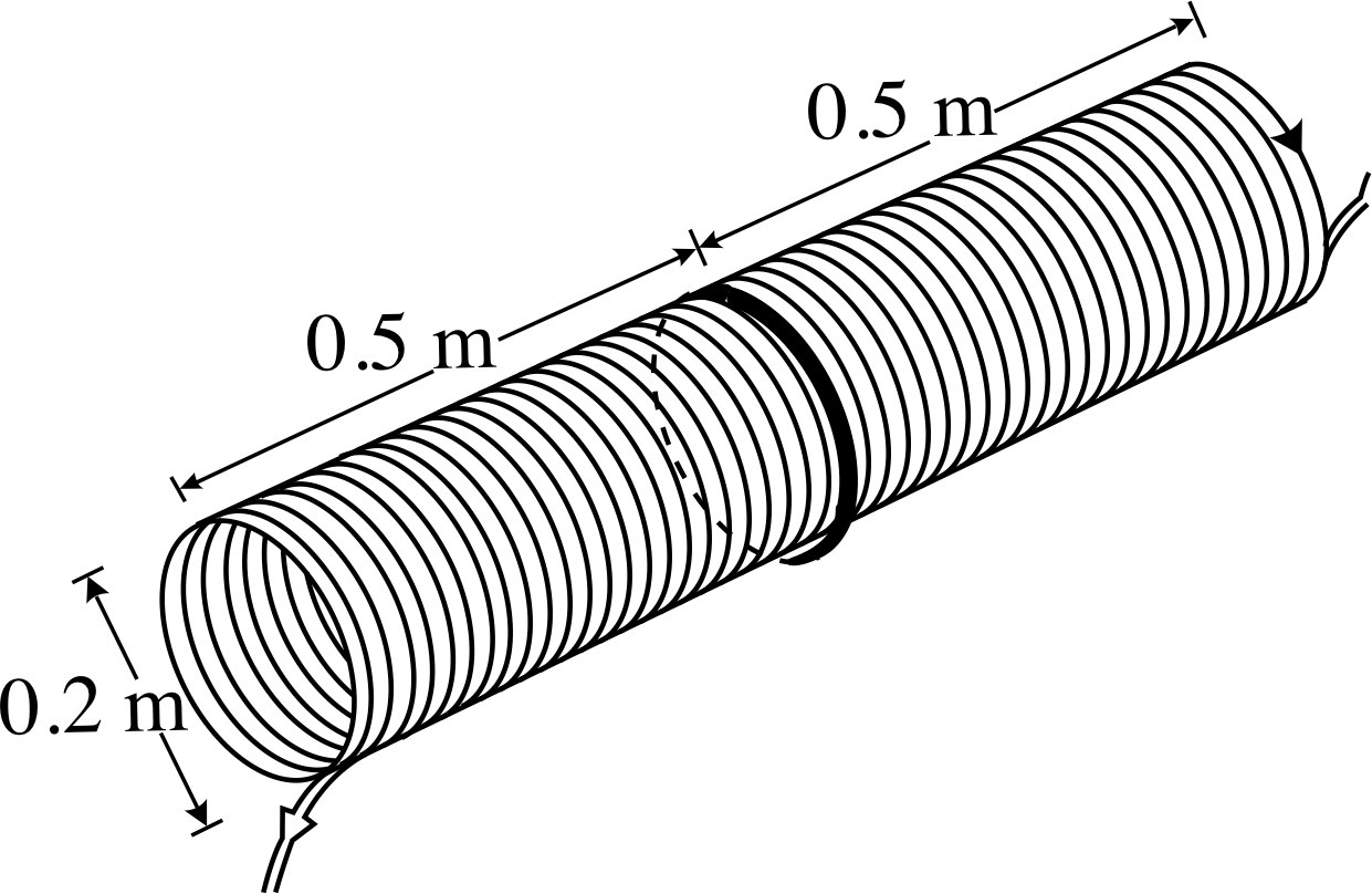
Figure 19 See Question T9.
The cylindrical solenoid shown in Figure 19 is of length 1 m and radius 0.1 m. It consists of 1000 turns of wire carrying a current of 1 A. A separate circular conducting loop, electrically insulated from the solenoid and carrying a current of 700 A has been wound around the middle of the solenoid so that it rests on top of the solenoid’s central loop. What is the magnetic field strength at the centre of the solenoid if the current in the separate loop flows (a) in the same direction and (b) in the opposite direction to the current in the solenoid?
(c) If the current in the solenoid always flows in the direction shown in Figure 19, what is the direction of the magnetic field at the centre of the solenoid for each of the cases described in (a) and (b)?
Answer T9
The field strength at the centre of the solenoid, due to the solenoid alone, is given by Equation 4,
$B_{\rm solenoid} = \dfrac{\mu_0NI}{L} = \dfrac{4\pi\times 10^{-7}\,{\rm T\,m\,A^{-1}\times 10^3\,m^{-1}\times 1\,A}}{1\,{\rm m}} = 1.26 \times 10^{-3}\,{\rm T}$
At the same point, the field due to the circular loop is given by Equation 3,
$B_{\rm loop} = \dfrac{\mu_0I}{2R} = \dfrac{4\pi\times 10^{-7}\,{\rm T\,m\,A^{-1}\times 700\,A}}{2\times 10^{-1}\,{\rm m}} = 4.40 \times 10^{-3}\,{\rm T}$
In case (a), the magnetic fields of the loop and the solenoid point in the same direction and the resulting field is of magnitude Bloop + Bsolenoid = 5.66 × 10⁻³ T. In case (b), the two fields are opposed and the resultant has magnitude Bloop − Bsolenoid = 3.14 × 10⁻³ T. (Note that we choose to take Bloop − Bsolenoid, not Bsolenoid − Bloop, to ensure that the magnitude of the resultant is positive.)
(c) Using the right–hand grip rule, and referring to Figure 19, we can see that in case (a) the total field points to the right and in (b) to the left.
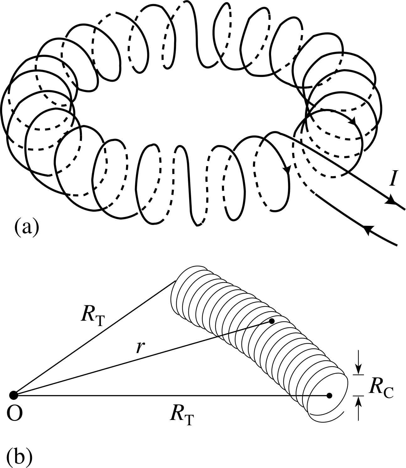
Figure 20 (a) A toroidal solenoid. (b) A section of a toroidal solenoid, having radius RT which is much larger than the coil turns radius RC.
We will consider one further current configuration. Suppose we take a long solenoid and curl it up so that the solenoid itself forms a single circular loop. This doughnut shape, shown in Figure 20a, is called a toroid or a torus and a coil wrapped around it is a toroidal solenoid. The magnetic field strength at a point which is within the coils of a toroidal solenoid (as shown in Figure 20b) and at a radial distance r from the centre of the toroid is:
Magnetic field strength at a point within a very long toroidal solenoid is:
$B_{\rm toroid}(r) = \dfrac{\mu_0NI}{2\pi r}$(5) i
where r is measured from the centre of the torus and N is the total number of turns on the solenoid. Figure 20b shows a very long toroidal solenoid, with the toroidal radius RT which is much larger than the coil turns radius RC.
Again, it is not appropriate here to prove Equation 5 but we can see that it is consistent with Equation 4,
$B_{\rm solenoid}= \dfrac{\mu_0NI}{L}$(Eqn 4)
for the case where RT ≫ RC. In such a case r ≈ RT and L = 2πRT ≈ 2πr and Equation 5 becomes the same as Equation 4. This might be expected for a toroidal solenoid of sufficiently large toroidal radius since an enlarged view of a small section of such a solenoid would appear to be almost straight and very long. We should not be surprised by this result for, after all, a toroidal solenoid is just a solenoid which has been made to join up with itself and might be thought of as having infinite length because it has no ends! Because the solenoid has no ends, the field does not ‘escape’ from the turns, and so the field outside an ideal uniformly–wound toroidal solenoid is zero.
Question T10
A toroidal solenoid with 200 turns has a radius of 10 cm, measured from the toroid centre to the centre of the solenoid turns, the latter having a radius of 2 cm. What are the maximum and minimum values of the magnetic field inside the coils when a current of 1.5 A flows through the wires? (You may treat this solenoid as long.)
Answer T10
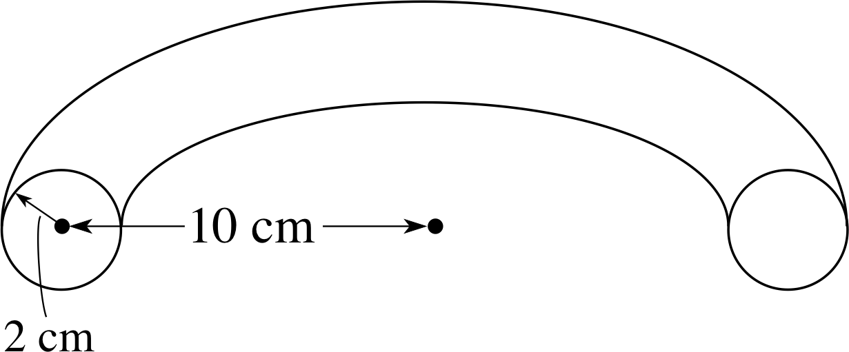
Figure 27 See Question T10.
We can use Equation 5,
$B_{\rm toroid}(r) = \dfrac{\mu_0NI}{2\pi r}$(Eqn 5)
to find the magnetic field strength within the turns of the solenoid at
various radial distances from the centre of the toroid as follows:
$B_{\rm toroid} = \dfrac{\mu_0NI}{2\pi r} = \dfrac{4\pi\times 10^{-7}\,{\rm T\,m\,A^{-1}\times 200\times 1.5\,A}}{2\pi r} = \dfrac{6\times 10^{-5}\,{\rm m}}{r}\,{\rm T}$
A cross section through the centre of the toroid (Figure 27) shows that the radial distances from the centre to the nearest and furthest points within the coils are 8 cm and 12 cm, respectively. Using these values for r then gives the two extreme values of field strength as 0.75 × 10⁻³ T and 0.50 × 10⁻³ T.
3.5 Summary of results for the fields produced by currents
Now we will summarize all the expressions for the magnitudes of the magnetic fields generated by simple current geometries.
Field strength at a radial distance r from a long straight wire
$B(r) = \dfrac{\mu_0I}{2\pi r}$(Eqn 2)
Field strength at the centre of a current loop of radius R
$B_{\rm loop} = \dfrac{\mu_0I}{2R}$(Eqn 3)
Field strength inside a long solenoid of N turns in a length L, far from the ends
$B_{\rm solenoid} = \dfrac{\mu_0NI}{L}$(Eqn 4)
Field strength within the turns of a long toroidal solenoid of N turns at a distance r from the toroid centre
$B_{\rm toroid}(r) = \dfrac{\mu_0NI}{2\pi r}$(Eqn 5)
To this collection, we will add one further useful result, stated without proof:
If we have a current carrying circuit of wire which includes a straight section, then there will be no contribution from that section to the magnetic field at any point along the projection of the axis of the straight section.
While we are not able to prove this final quoted result now we can make it reasonable by the following argument. Movement of electric charge constitutes a current and it is this current which gives rise to magnetic fields. Imagine an observer positioned in line with a current flowing towards or away from the observer. The charge flow has no velocity component across the line of sight and the observer will therefore be unaware of the motion of the charge and will observe no magnetic field.
The boxed results above, together with the principle of superposition, allow us to deduce the magnetic field produced by various configurations of current, provided they can be related to the simple situations discussed above. We will end this subsection by giving an example of this technique.
Example 1
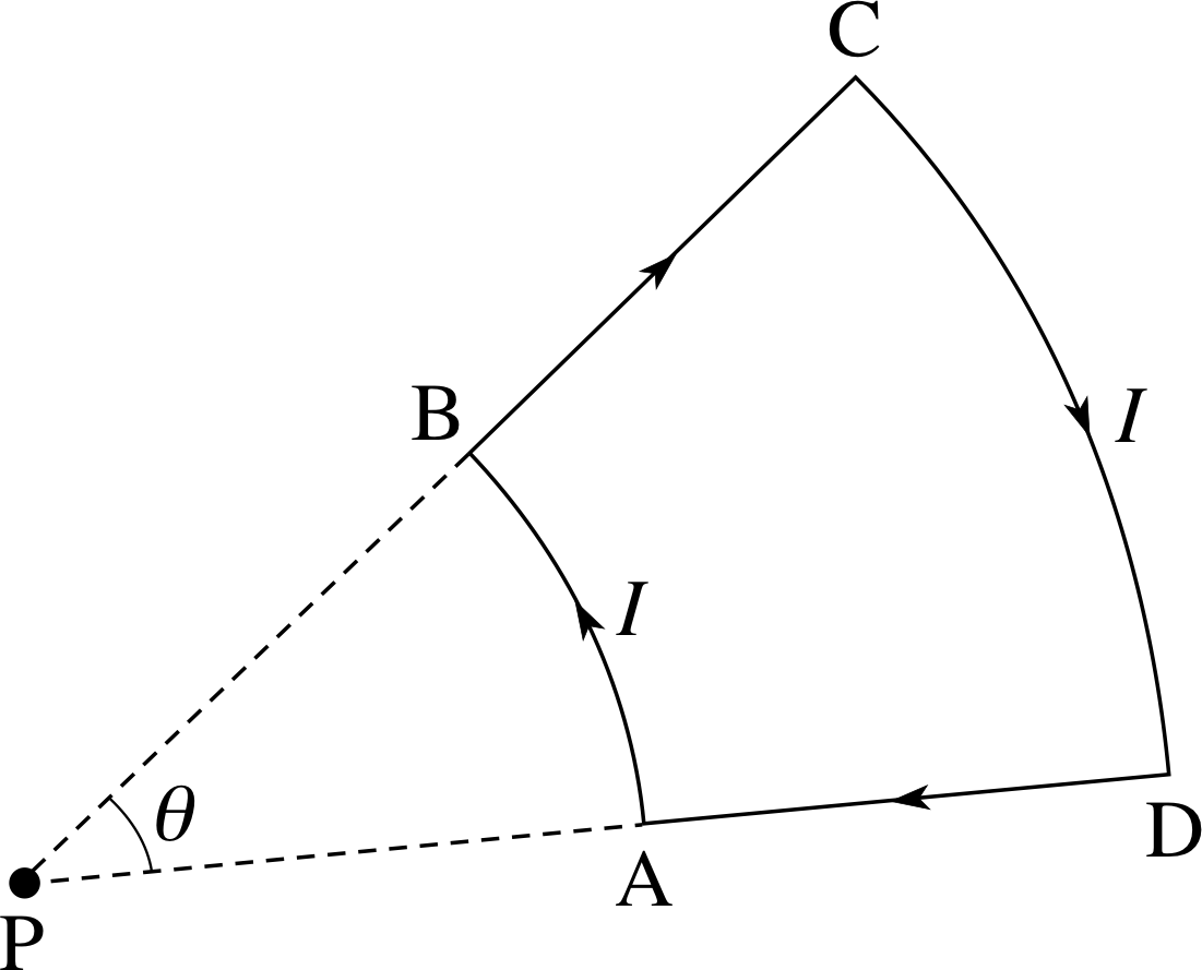
Figure 21 A circuit composed of straight and circular sections.
A wire loop, carrying a current I, has the shape shown by the solid lines in Figure 21. Find an expression for the magnetic field at the point P.
Solution
From Figure 21, we see that there are two straight sections of wire (DA and BC) in which the current is directed towards and away from the point P. The currents in these sections produce no magnetic field at P. The two circular segments AB and CD both subtend the same angle θ at P. We can take the logical step of saying that if a full turn of a circular loop produces a certain value of field at the centre of the loop, then the fraction θ/2π of the loop produces that fraction of the field. i The fields from the two current segments will oppose one another (as the currents are in opposite directions), and that of the nearer segment, AB, will be the stronger so that the resultant field will be pointing out of the page at P.
From Equation 3,
$B_{\rm loop} = \dfrac{\mu_0I}{2R}$(Eqn 3)
its magnitude B is found to be given by
$B_{\rm net} = \dfrac{\theta}{2\pi}\left(\dfrac{\mu_0I}{2R_1}-\dfrac{\mu_0I}{2R_2}\right) = \dfrac{\mu_0I\theta}{4\pi}\left(\dfrac{1}{R_1}-\dfrac{1}{R_2}\right)$
where R1 is the radius of arc AB and R2 is the radius of arc CD.
3.6 The electromagnet
Several times in this module we have referred to the fact that a magnet can be made using electric currents. In the sense that a coil or solenoid carrying a current produces a magnetic field, these devices behave as magnets. We can dramatically increase the magnetic strength of such a device by wrapping the coil or solenoid around a core of ferromagnetic material, such as iron. Such a device is said to be an electromagnet.
In an electromagnet the current produces a magnetic field and this in turn induces strong magnetism in the ferromagnetic material within the coil or solenoid. This induced magnetism then enhances considerably the magnetic forces from the coil or solenoid alone. If the ferromagnetic material is magnetically soft then when the current ceases so too does the magnetism, although a small amount may remain in the ferromagnetic material to the extent that it is not fully soft. The flexibility of the electromagnet, as opposed to a permanent magnet, is that its strength is variable and controllable. Electromagnets have very widespread applications, ranging from tiny earphones to huge cranes for lifting magnetic materials. If the ferromagnetic material within a coil is magnetically hard then the material may become permanently magnetized. i
4 Closing items
4.1 Module summary
- 1
-
There are many examples of everyday applications of magnetism, including the use of the magnetic compass in navigation.
- 2
-
The centres of magnetic force in a bar magnet are located near the ends of the magnet and are known as the poles of the magnet. A freely–suspended bar magnet aligns itself north–south, and its poles are known as the north and south poles. Two unlike poles attract each other and two poles of the same polarity repel each other. At any point (x, y, z) the magnetic field B (x, y, z) relates the magnetic force Fmag on a moving charged particle to the charge q of the particle and its velocity υ. The direction of the field at any point indicates the direction in which an isolated north magnetic pole placed at that point would tend to move (or the direction in which the north pole of a freely suspended compass needle would point). The magnitude of the field at any point may be determined by measuring the magnitude Fmag of the magnetic force that would act on a particle of charge q as it moves through the point (x, y, z), in a direction at right angles to the magnetic field, with a speed υ⊥
$B(x, y, z) = \dfrac{F_{\rm mag} \text{(on }q\text{ as it moves through the point }(x, y, z))}{q\upsilon_{\perp}}$(1)
- 3
-
The SI unit of magnetic field is the tesla (T) where 1 T = 1 N s C−1 m−1.
- 4
-
An elementary description of the Earth’s magnetic field is that it is similar to the field of a bar magnet, oriented such that its magnetic south pole points towards the Earth’s geographic North Pole.
- 5
-
A magnetic field may be depicted by field lines. Such lines are drawn so that the field is tangential to the field line at any point and has the same direction as the field line at that point. The density of the field lines in any region is proportional to the magnitude of the magnetic field in that region. (In practice this last requirement is sometimes ignored, for the sake of simplicity.) Plots of the field patterns of various orientations and arrangements of magnets can be obtained using a compass needle.
- 6
-
Magnetic poles are invariably found in pairs of opposite polarity. An isolated pair of poles of equal strength but opposite polarity, separated by a small distance, is known as a magnetic dipole. There is no evidence for the existence of isolated magnetic monopoles.
- 7
-
Materials can be simply classified into two groups: those attracted by a magnet and those not attracted by a magnet. Materials in the first group (ferromagnetic materials) can be further classified as magnetically hard or magnetically soft. Permanent magnets are made from magnetically hard materials.
- 8
-
Oersted’s experiments on the deflection of a compass needle by electric currents were the first to demonstrate the connection between electric currents and magnetic fields. The lines of the magnetic field produced by a current in a straight wire are concentric circles about the current, hence explaining Oersted’s results. The right-hand grip rule gives the direction of the magnetic field produced by a current in a straight wire.
- 9
-
Formulae are available which give the strength of the magnetic fields produced in certain specified locations in the vicinity of currents in: a straight wire, a circular loop and a multi–turn coil, a long solenoid and a long toroidal solenoid
Field strength at a radial distance r from a long straight wire
$B(r) = \dfrac{\mu_0I}{2\pi r}$(Eqn 2)
Field strength at the centre of a current loop of radius R
$B_{\rm loop} = \dfrac{\mu_0I}{2R}$(Eqn 3)
Field strength inside a long solenoid of N turns in a length L, far from the ends
$B_{\rm solenoid} = \dfrac{\mu_0NI}{L}$(Eqn 4)
Field strength within the turns of a long toroidal solenoid of N turns at a distance r from the toroid centre
$B_{\rm toroid}(r) = \dfrac{\mu_0NI}{2\pi r}$(Eqn 5)
- 10
-
It is the electrons within the constituent atoms of materials which generate their magnetic properties.
- 11
-
Electromagnets are made by winding a coil or a solenoid around a core of magnetically soft ferromagnetic material.
4.2 Achievements
Having completed this module, you should be able to:
- A1
-
Define the terms that are emboldened and flagged in the margins of the module.
- A2
-
Describe and sketch the form of the Earth’s magnetic field, and explain the use of an inclinometer to measure the angle of inclination or dip.
- A3
-
Describe the interactions which arise between like and unlike poles.
- A4
-
Describe how the magnitude and direction of a magnetic field can be determined at any point, and explain how information about magnetic fields can be obtained using a compass. Describe how field lines may be used to indicate the strength and direction of a magnetic field. Describe and illustrate the form of the field patterns produced by bar magnets in various orientations.
- A5
-
Describe the broad categorization into magnetic and non–magnetic materials and the division of magnetic materials into hard and soft; describe further categorizations, including that of ferrites.
- A6
-
Describe Oersted’s experiments, concerning the deflection of a compass needle near an electric current, and explain the results in terms of the magnetic field produced by a current in a long straight wire.
- A7
-
Describe and draw the field pattern produced by a current in a straight wire; state and use the right–hand grip rule to determine the field direction at a point near the wire.
- A8
-
Use the field pattern of a straight wire to predict patterns for other simple wire configurations and, in particular, to reproduce patterns associated with loops, coils, solenoids and toroids.
- A9
-
Recognize and use formulae which give the magnetic field strength at certain locations near the wire configurations in Achievements A7 and A8 and justify that these formulae are physically plausible.
- A10
-
Use the principle of superposition to calculate resultant field strengths in regions where there is more than one source of magnetic field.
Study comment You may now wish to take the Exit test for this module which tests these Achievements. If you prefer to study the module further before taking this test then return to the topModule contents to review some of the topics.
4.3 Exit test
Study comment Having completed this module, you should be able to answer the following questions each of which tests one or more of the Achievements.
Question E1 (A2)
How does the angle of inclination or dip vary as the point of observation moves over the Earth’s surface from the magnetic pole in the southern hemisphere to that in the northern hemisphere? Over what parts of the Earth’s surface would you expect to find zero angle of dip?
Answer E1
The angle of dip is the angle between the Earth’s magnetic field and the horizontal. At the south magnetic pole, the magnetic field points vertically upwards, i.e. the angle of dip is 90° above the horizontal (so angle of inclination is a better term than angle of dip, particularly in the southern hemisphere). Moving from the south to the north magnetic pole, the angle of inclination rotates smoothly through 180° to point 90° below the horizontal, passing through zero inclination midway between the magnetic poles. Points of zero inclination will encircle the Earth at (approximately) halfway between north and south magnetic poles, thus defining a magnetic equator. (This picture of the Earth’s field is somewhat idealized. In practice, there are local variations in the field, so the change from N to S is not completely smooth.)
(Reread Subsections 2.2 and 2.3 if you had difficulty with this question.)
Question E2 (A3, A4 and A7)
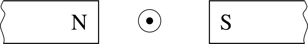
Figure 22 See Question E2.
Figure 22 shows a wire carrying a current out of the plane of the paper, placed between the poles of two bar magnets. (a) State whether the two bar magnets are attracting or repelling each other. (b) Sketch the resultant magnetic field pattern due to the bar magnets and the current.
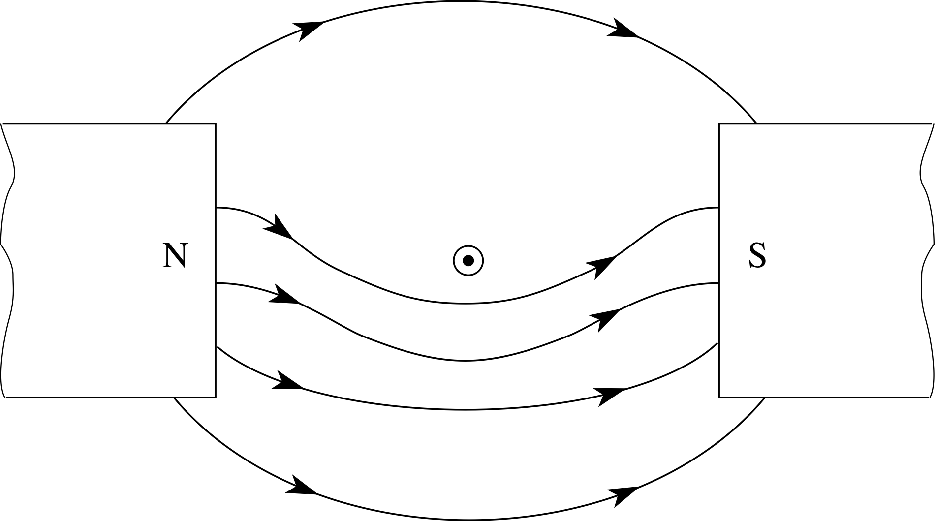
Figure 28 See Answer E2.
Answer E2
(a) The poles are unlike, so they attract each other.
(b) See Figure 28. The field lines due to the current alone are anticlockwise in the diagram, and those from the bar magnets alone are directed from left to NS right in the diagram, so above the wire the fields tend to cancel each other, while below the wire they reinforce each other, producing a stronger field below the wire and a weaker field above the wire.
(Reread Subsections 2.2, 2.3 and 3.2 if you had difficulty with this question.)
Question E3 (A6 and A7)
Electrical apparatus is often connected to a power supply using a live and a return wire, carrying the current, and an earth wire, carrying no current, bound together in a single three–core cable. What effect does this arrangement have on the magnetic fields generated by the currents in the two current carrying wires?
[Hint: You are not required to include the earth wire in your discussion.]
Answer E3
The current in each wire will produce a magnetic field around the wire in the sense given by the right–hand grip rule. Since the two currents are in opposite directions, the two fields are in opposite directions. If these currents in the two wires are equal in magnitude and opposite in direction and the two wires are straight and are superimposed on one another, then the two fields will completely cancel one another since they have the same magnitude and opposite directions. Sometimes the two insulated wires are twisted together, in which case their magnetic fields cannot exactly cancel, but at large distances from the wires (i.e. large in comparison with the separation of the wires) this difference between the field magnitudes is negligible and the net field will be close to zero. (Twisting the wires is a simple and effective way of keeping two single wires close together.)
(Reread Subsection 3.2 if you had difficulty with this question.)
Question E4 (A6 and A9)
A long straight wire carries a current of 8 A. Calculate the strength of the magnetic field produced at distances of 5, 10, 20 and 50 mm from the wire. Sketch a graph to show how field strength varies with radial distance from the wire.
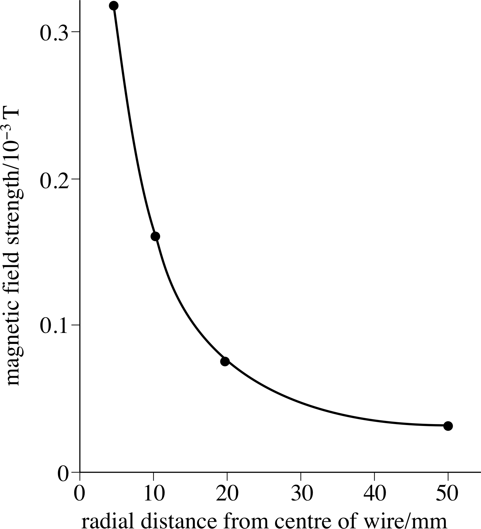
Figure 29 See Answer E4.
Answer E4
From Equation 2,
$B(r) = \dfrac{\mu_0I}{2\pi r} = \dfrac{4\pi\times 10^{-7}\,{\rm T\,m\,A^{-1}}\times 8\,{\rm A}}{2\pi r} = \left(\dfrac{1.6\times 10^{-6}\,{\rm m}}{r}\right)\,{\rm T}$
Substituting r = 5, 10, 20 and 50 mm into this equation gives magnetic field strengths of 0.32 × 10⁻³ T, 0.16 × 10⁻³ T, 0.08 × 10⁻³ T and 0.032 × 10⁻³ T, respectively. Magnetic field strength as a function of radial distance from a long straight wire carrying a current of 8 A is plotted in Figure 29.
(Reread Subsection 3.2 if you had difficulty with this question.)
Question E5 (A9 and A10)
A wire of length L carries a current I. Compare the strengths of the central magnetic fields produced when this length of wire is formed into (a) a single circular loop, (b) a circular coil of n turns. (c) If more of this same wire were available, how many turns of the loop in (a) would be required to produce the field obtained in (b)?
Answer E5
(a) When a wire of length L is bent into a circle, its radius R may be obtained from the equation for the circumference of a circle: 2πR = L. If a current I flows in this wire then, from Equation 3,
$B_{\rm loop} = \dfrac{\mu_0I}{2R}$(Eqn 3)
the field at the centre of the loop is Bloop = μ0Iπ/L.
(b) When the same length of wire is curled up to make n circular turns, their radius will be reduced to L/(2πn), i.e. by a factor of n compared with (a). Also, from a given length of wire, the number of turns has been increased by a factor of n. So the field strength at the centre will have increased by a factor of n2 and the new field strength is μ0n2Iπ/L.
(c) To increase the central field to this value, but still keeping the original radius, would require n2 turns.
(Reread Subsection 3.3 if you had difficulty with this question.)
Question E6 (A8, A9 and A10)
A large even number of long straight parallel wires, each carrying the same current in the same sense, are arranged symmetrically at equal spacings around the circumference of a cylinder parallel to the axis of the cylinder. Describe the magnetic field generated by these currents (a) in the regions inside and (b) outside the cylinder.
Answer E6
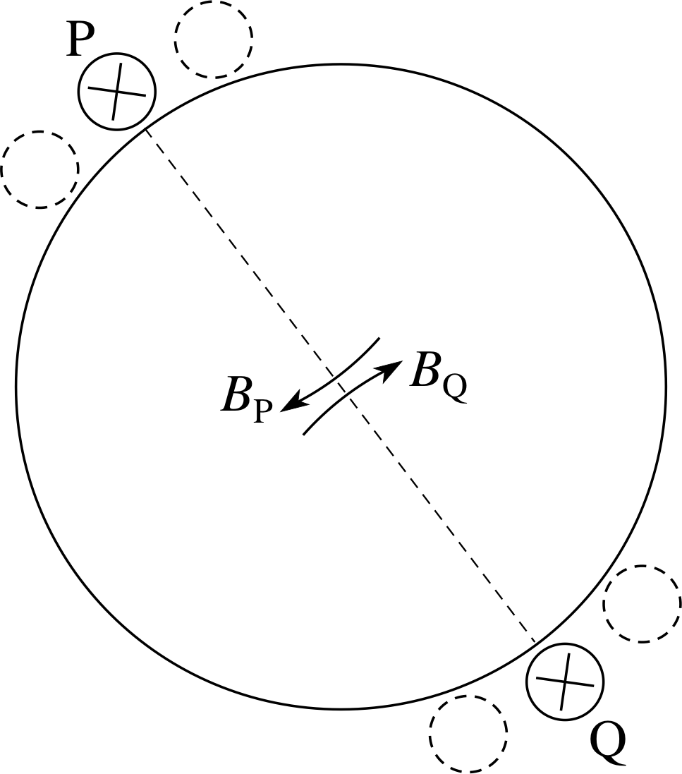
Figure 30 See Answer E6.
(a) All the wires carry the same current and are at the same distance from the axis of the cylinder. The magnitude of the component of magnetic field produced at this axis by eachcurrent will therefore be the same. The direction of a field component will be perpendicular to the line joining the wire which produces it and the axis, and will lie in a cross–sectional plane through the cylinder. Thus the field component BP produced by wire P, will be equal and opposite to the field component BQ produced by the symmetrically placed wire Q on the opposite side of the cylinder (see Figure 30). As there is an even number of wires, there will be a net zero field along the axis. At other internal points however the field will not be zero. This same analysis would be valid if the current were to flow uniformly down the outer surface of a conducting cylinder; the field on axis would be zero.
(b) At points outside the cylinder and at distances large in comparison with the cylinder diameter, the magnetic field strength will be approximately the same as that from a single long straight wire carrying a current equal to the total current carried by all the wires on the cylinder. Nearer to the cylinder, the field could be found from a vector sum of the field components from all the wires.
(Reread Subsection 3.2 if you had difficulty with this question.)
Study comment This is the final Exit test question. When you have completed the Exit test go back and try the Subsection 1.2Fast track questions if you have not already done so.
If you have completed both the Fast track questions and the Exit test, then you have finished the module and may leave it here.
Study comment Having seen the Fast track questions you may feel that it would be wiser to follow the normal route through the module and to proceed directly to the following Ready to study? Subsection.
Alternatively, you may still be sufficiently comfortable with the material covered by the module to proceed directly to the Section 4Closing items.