PHYS 4.4: Electromagnetic induction |
PPLATO @ | |||||
PPLATO / FLAP (Flexible Learning Approach To Physics) |
||||||
|
1 Opening items
1.1 Module introduction
Our modern world would be impossible without electromagnetic induction – the phenomenon that underlies the operation of many devices, including power station generators, microphones, tape recorders, bicycle dynamos, car alternators, ignition systems and speedometers.
In Section 2 we begin our discussions with some examples of electromagnetic induction that are easy to demonstrate using simple apparatus – by moving a wire in a magnetic field, or by moving or varying the magnetic field around a circuit. These operations generate an induced voltage. Energy conservation allows us to deduce the polarity of the induced voltage and this is formalized and generalized in a statement of Lenz’s law.
Section 3 introduces Faraday’s law of electromagnetic induction, which relates the magnitude of an induced voltage to the rate of change of the magnetic flux linking a circuit. Faraday’s law enables us to measure an unknown magnetic field using a search coil, and to explain the generation of electricity in an alternator or a dynamo.
Section 4 is about the behaviour of a transformer and an induction coil. It introduces the coefficients of self inductance and of mutual inductance between two circuits.
In Section 5 we deal with motional induction for a single conductor and predict the induced voltage using both Faraday’s law and the Lorentz force. We end with some further examples of induction, including the homopolar generator and the production and avoidance of eddy currents.
Study comment Having read the introduction you may feel that you are already familiar with the material covered by this module and that you do not need to study it. If so, try the following Fast track questions. If not, proceed directly to the Subsection 1.3Ready to study? Subsection.
1.2 Fast track questions
Study comment Can you answer the following Fast track questions? If you answer the questions successfully you need only glance through the module before looking at the Subsection 6.1Module summary and the Subsection 6.2Achievements. If you are sure that you can meet each of these achievements, try the Subsection 6.3Exit test. If you have difficulty with only one or two of the questions you should follow the guidance given in the answers and read the relevant parts of the module. However, if you have difficulty with more than two of the Exit questions you are strongly advised to study the whole module.
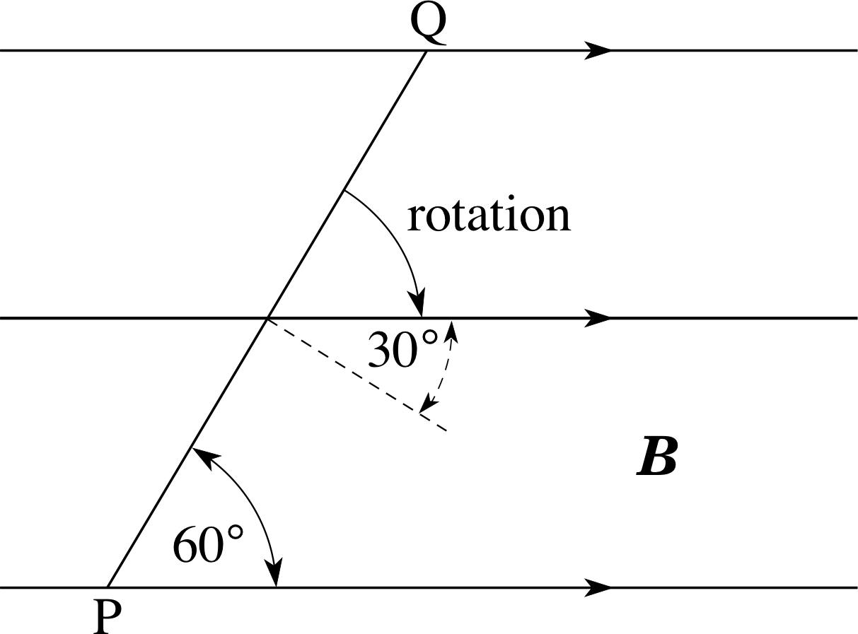
Figure 1 See Question F1.
Question F1
A rectangular coil of 50 turns has dimensions 14.0 cm × 30.0 cm and an electrical resistance R = 2.0 Ω. The plane of the coil PQ is quickly rotated from a position in which it makes an angle of 60° with a magnetic field to a position in which its plane is parallel to the field (Figure 1). If the field strength is B = 0.40 T, calculate the total charge which circulates around the coil.
Answer F1
The flux initially linking the coil, area A, is Φ = NBA cos 30°. After the rotation there is no flux linking the coil, so the flux change is then ∆Φ = NBA cos 30°. The magnitude of the average induced voltage
$\langle V_{\rm ind}\rangle = \dfrac{\Delta{\it\Phi}}{\Delta t} = \langle I\rangle R = R\dfrac{\Delta q}{\Delta t}$
where $\langle I\rangle$ is the average current and ∆q is the total charge that flows. We see that ∆q = ∆Φ/R and so:
∆q = NBA cos 30°/R = 50 × 0.40 T × 0.14 m × 0.30 m × cos 30°/2.0 Ω = 0.36 C
Question F2
A flywheel of radius 1.3 m, with its plane vertical and its axis in a north–south direction, rotates at 240 revolutions per minute, clockwise when viewed from the south. If the Earth’s magnetic field is 48.5 × 10⁻⁶ T, inclined downwards at 69.6° to the horizontal and directed 8° west of north, calculate the magnitude and polarity of the voltage induced between the axle and the outer rim of the flywheel.
Answer F2
The induced voltage has magnitude Vind = BAf where B is the magnetic field component at right angles to the plane of the wheel, A the area of the wheel and f the rotation frequency, i.e. 4 Hz.
The horizontal component of magnetic field, Bh, has magnitude
Bh = 48.5 × 10⁻⁶ T × cos 69.6°
and its component due north (perpendicular to the wheel) has magnitude
Bh cos 8° = 48.5 × 10⁻⁶ T × cos 69.6° × cos 8° = 1.67 × 10⁻⁵ T
henceVind = 1.67 × 10⁻⁵ T × π × (1.3 m)2 × 4.00 Hz = 3.5 × 10⁻⁴ V
The Lorentz force on an imagined positive charge within the flywheel would be radially outwards, (or radially
inwards on a free electron in the material) so the rim will develop a positive potential with respect to the axle.
1.3 Ready to study?
Study comment In order to study this module, you will need to be familiar with the concepts of charge, current, electrical potential energy, electrical power and potential difference and the relationships between these, including Ohm’s law. You should be familiar with the concept and use of magnetic field, magnetic poles, magnetic field lines and the form of the magnetic field produced by a long straight wire, a solenoid and a bar magnet. It is assumed that you have met the vector statement of the Lorentz force (electromagnetic force) on a charged particle moving in a magnetic field and an electric field, and that you are familiar with a rule such as right–hand rule or the corkscrew rule for working out the direction of that force (see Question R2). Also, you will need to be familiar with the principle_of_conservation_of_mechanical_energyprinciple of conservation of energy and the use of the equations describing uniform acceleration and uniform circular motion. Mathematical techniques assumed are the use of vectors, resolution into component vectors and the use of calculus notation, such as dA/dt (the rate of change of A with respect to t). The derivatives of trigonometric functions are used but these will be introduced when needed. If you are uncertain about any of these terms you can review them now by referring to the Glossary, which will also indicate where they are developed in FLAP. The following questions will allow you to decide whether you need to review some of the topics before embarking on this module.
Question R1
At a certain point on the Earth’s surface, the horizontal component of the Earth’s magnetic field has strength 42 μT i and is directed 10° west of geographical north. Draw a diagram showing the north–south and east–west components_of_a_vectorcomponents of the Earth’s magnetic field at this point.
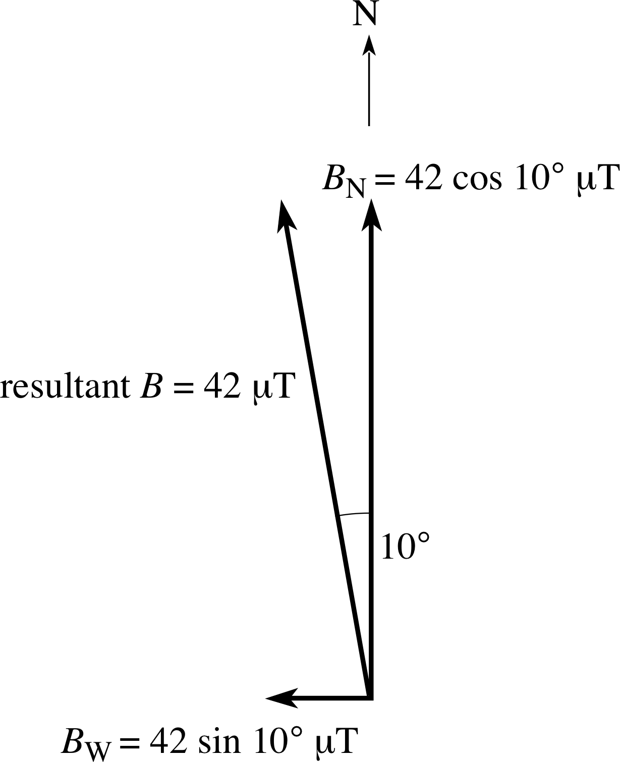
Figure 25 See Answer R1.
Answer R1
The components and the resultant_vectorresultant field are shown in Figure 25. (This figure is to scale.) Consult magnetic field in the Glossary for further information.
Question R2
Sketch the magnetic field lines around (a) a bar magnet and (b) a current carrying solenoid. In (b) show the directions of the current and the field.
(c) Calculate the magnetic field strength inside a solenoid of N = 600 turns, of length l = 0.80 m which carries a current I = 1.2 A. i
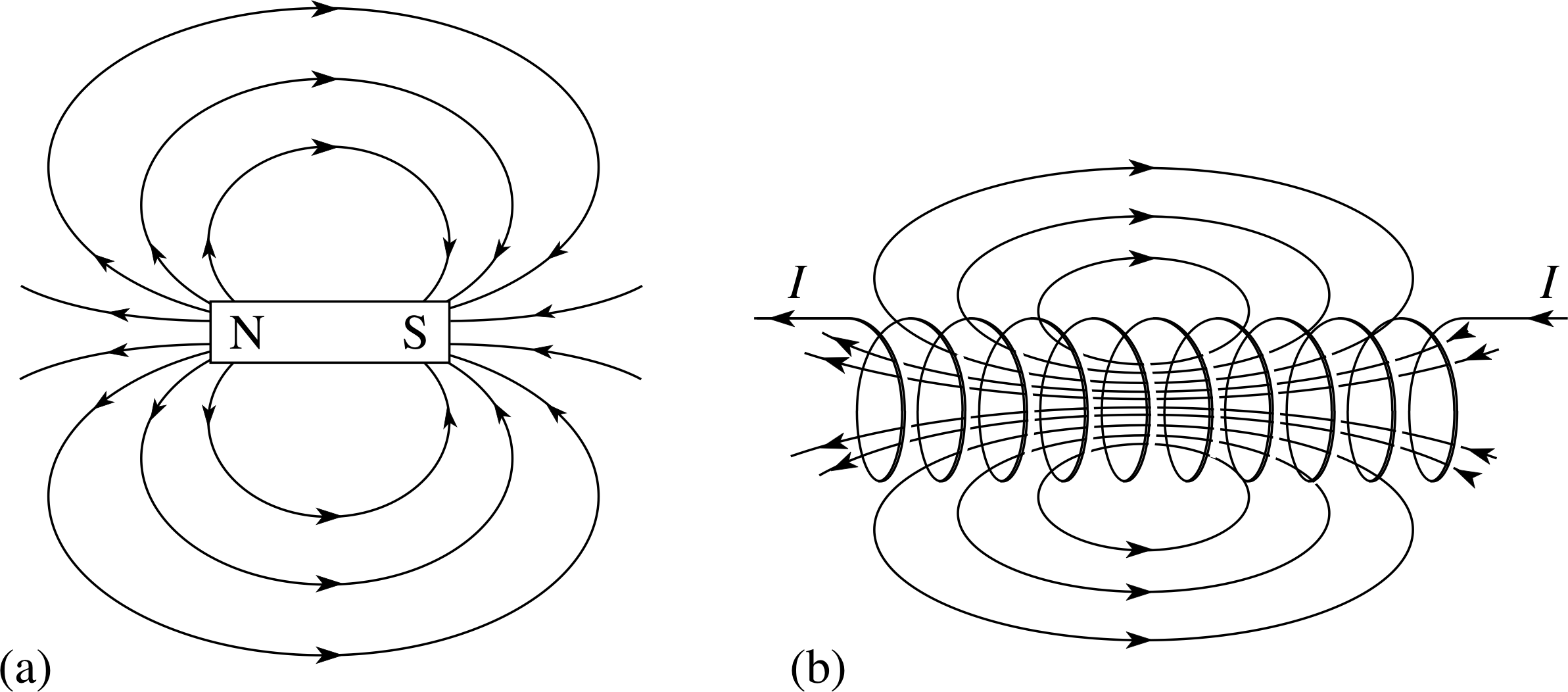
Figure 4 The magnetic field lines around (a) a bar magnet (as in Figure 2) and (b) a current carrying solenoid (as in Figure 3). The coil is wound in an anticlockwise direction. Note that field lines are directed from N to S, and they curl around a current in the same sense that the fingers of your right hand curl around your thumb when you grip something.
Answer R2
(a) and (b) The field lines around a bar magnet and solenoid are shown in Figure 4. The direction of the field lines in (b) may be found by applying the right–hand grip rule to a portion of the wire that makes up one of the coils. To do this point the thumb of your right hand in the direction of the current. The fingers of your right hand then curl around the thumb in the same sense that the magnetic field lines curl around the current.
(c) The field inside a solenoid (well away from the end) is uniform and for a long solenoid of length l with N turns and carrying a current I has magnitude:
$B = \dfrac{\mu_0NI}{l} = \rm \dfrac{4\pi\times10^{-7}\,T\,m\,A^{-1}\times600\times1.2\,A}{0.80\,A} = 1.1\times10^{-3}\,T$
Consult currents and magnetic fields in the Glossary for further information.
Question R3
A particle of charge q = 2.0 × 10⁻¹⁰ C is in a uniform electric field of strength E = 3.0 × 10⁴ N C−1, which accelerates the particle through a distance of 40 mm. Calculate (a) the potential difference between the starting and finishing points of the particle’s journey, and (b) the change in the particle’s electrical energy.
Answer R3
(a) Field strength E = 3.0 × 10⁴ N C−1 = 3.0 × 10⁴ V m−1. The potential difference over a distance d of 40 mm is
V = Ed = 3.0 × 10⁴ V m−1 × 4.0 × 10−2 m = 1.2 × 10³ V
This is equivalent to 1.2 × 10³ J C−1, since 1 V = 1 J C−1.
(b) Energy change = qV = 2.0 × 10−10 C × 1.2 × 103 J C−1 = 2.4 × 10⁻⁷ J
Consult electric field and electric potential in the Glossary for further information.
Question R4
Write down a vector expression for the Lorentz force F on a charge q moving with velocity υ through a region containing an electric field E and a magnetic field B. Calculate the magnitude and state the direction of this force on a proton moving with a speed υ = 3.0 × 10⁶ m s−1 eastward in a magnetic field of magnitude B = 52 μT, directed northwards. i
Answer R4
The Lorentz force on q is given by: F = q (E + υ × B) where υ × B is the vector (or cross) product of υ and B. When a proton with q = e moves at right angles to the magnetic field with a speed υ, and when E = 0, it
experiences a force of magnitude F = eυB. So:
F = 1.602 × 10−19 C × 3.0 × 106 m s−1 × 52 × 10−6 T = 2.5 × 10⁻¹⁷ N
The magnetic force is Fmag = qυ × B and the corkscrew rule or the right–hand rule then gives the force on the positive charge as being vertically upwards.
Consult electromagnetic force and the Lorentz force law in the Glossary for further information.
Question R5
A rectangular coil, of width 4.0 cm and height 8.0 cm, rotates at 300 revolutions per minute about a vertical central axis in its plane. Calculate (a) the area of the coil in m2, (b) the angular speed of the coil in rad s−1, and (c) the linear speed of one of its sides in m s−1.
Answer R5
(a) Area of coil = height × width = 8.0 × 10−2 m × 4.0 × 10−2 m = 3.2 × 10⁻³ m2
(b) Angular speed ω = 2πf, where f = frequency.
If f = 300 revolutions per minute = 5.00 revolutions per second = 5.00 Hz, then ω = 10.0π rad s−1 = 31.4 rad s−1. (c) Linear speed υ = rω. Since the radius of circular motion
r = a/2 = 2.0 cm, then
υ = 2.0 × 10−2 m × 31.4 rad s = 0.63 m s−1
Consult circular motion in the Glossary for further information.
2 Introducing electromagnetic induction
2.1 Experiments with circuits and magnets
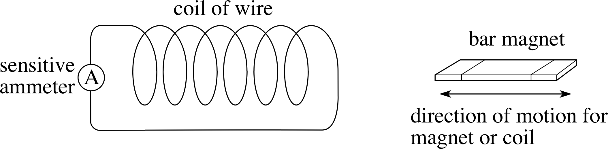
Figure 2 Relative motion between a magnet and a circuit.
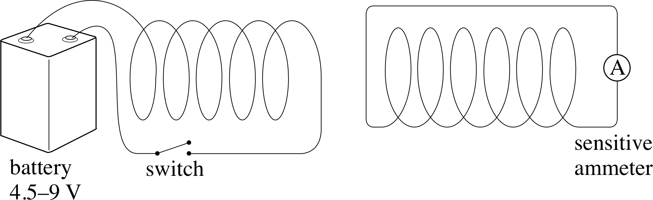
Figure 3 Changing the current in a nearby circuit.
Figure 4 The magnetic field lines around (a) a bar magnet (as in Figure 2) and (b) a current carrying solenoid (as in Figure 3). The coil is wound in an anticlockwise direction. Note that field lines are directed from N to S, and they curl around a current in the same sense that the fingers of your right hand curl around your thumb when you grip something.
The best way to start learning about electromagnetic induction is to see it in action – Figures 2 and 3 show some suitable simple demonstrations. If you have the opportunity you might like to try these if you have not already seen them. i
For the case shown in Figure 2, the magnet is moved at various speeds in and out of the coil or is moved around within the coil, or the magnet is held steady while the coil is moved.
In the case of Figure 3 both coils are stationary and the effect of opening or closing the switch is observed. In either case the sensitive ammeter will show that a current flows in the circuit to which it is attached.
In such demonstrations you will find that the common feature required to produce a deflection on the meter is that something is changing.
In each case, the change involves a magnetic field. The more rapid the change, the greater the deflection seen on the ammeter, and if the change is reversed the meter deflection is also reversed. In Figure 2, the field is that of the bar magnet, and in Figure 3 it is that due to the coil in the battery circuit (on the left) which acts as an electromagnet when a current flows through it.
If you picture the magnetic field lines of these two magnets (Figure 4) you will see that each method of producing a meter reading involves changing the number of field lines that thread through the coil in the meter circuit. In the case of Figure 2 the change is caused by the relative motion of the magnet and coil, while in Figure 3 the change is caused by an alteration in the current supplied to the electromagnet, but in both cases the immediate cause of the deflection is the change in the number of magnetic field lines threading the meter circuit.
In both these examples the current which flows through the meter circuit, produced by the changing magnetic field in the region around the circuit, is called an induced current. We associate the flow of currents in any circuit with a potential difference, or voltage, so we infer that, while the field is changing, it is as though a temporary power supply were driving charge around the circuit, and we say there is an induced voltage in the circuit. i There will only be an induced current in response to the induced voltage if there is a complete circuit through which the current can flow – but the induced voltage can exist even when the meter circuit is incomplete and there is no an induced current. In this sense, the induced voltage is the more fundamental phenomenon. The process by which these induced voltages are produced is called electromagnetic induction.
The size of the induced voltage between two given points will generally increase with the rapidity of the change that causes it. Moreover, that induced voltage may be positive or negative, depending on which of the points is at the higher voltage. This sign is is said to determine the polarity of the induced voltage. It is generally the case that reversing the change will produce an induced voltage of opposite polarity.
Aside Some authors use the term induced e.m.f. (electromotive force) rather than induced voltage. In FLAP we refrain from using that term to avoid the misconception that the quantity involved is a force. The quantity is a potential difference, not a force.
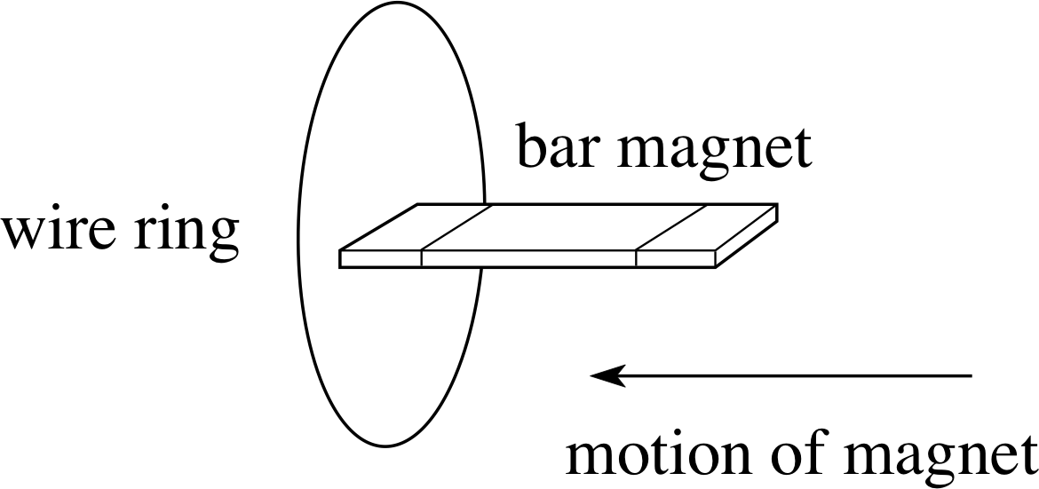
Figure 5 Inducing a current in a wire ring.
In Figures 2 and 3 you can think of the coil in the meter circuit as acting like a voltage generator, whilst the field is changing, with its ends as the generator terminals and the induced voltage as the potential difference between them, but this picture can sometimes be unhelpful. For example, in Figure 5, moving the magnet induces a current in the wire, but now the ‘coil’ consists of a single ring of wire and there is no obvious location for the generator.i
It is often better to think of electromagnetic induction as something that takes place throughout a circuit, and to think in terms of induced potential differences or voltages being produced between any two points in the circuit. The induced current and voltage are related via the circuit resistance – just as current and voltage are related by Ohm’s law in a d.c. circuit. Thus, in a circuit of total resistance R, an induced voltage Vind will produce an induced current Iind where
$I_{\rm ind} = \dfrac{V_{\rm ind}}{R}$(1)
Electromagnetic induction is an important phenomenon with many useful applications. However, there is also a situation where an induced voltage in a circuit is particularly troublesome. This is where fluctuating magnetic fields (e.g. from a.c. mains currents nearby) produce unwanted voltages in a circuit. This phenomenon is called electromagnetic pick–up. Often a great deal of trouble is taken to avoid this problem, for example by screening out the fields or by careful electrical grounding of the circuits and the electrical equipment.
We can summarize this introductory subsection as follows:
Electromagnetic induction is a process by which a changing magnetic field causes an induced voltage. The more rapid the change, the greater the voltage. The direction of the change determines the polarity of the voltage.
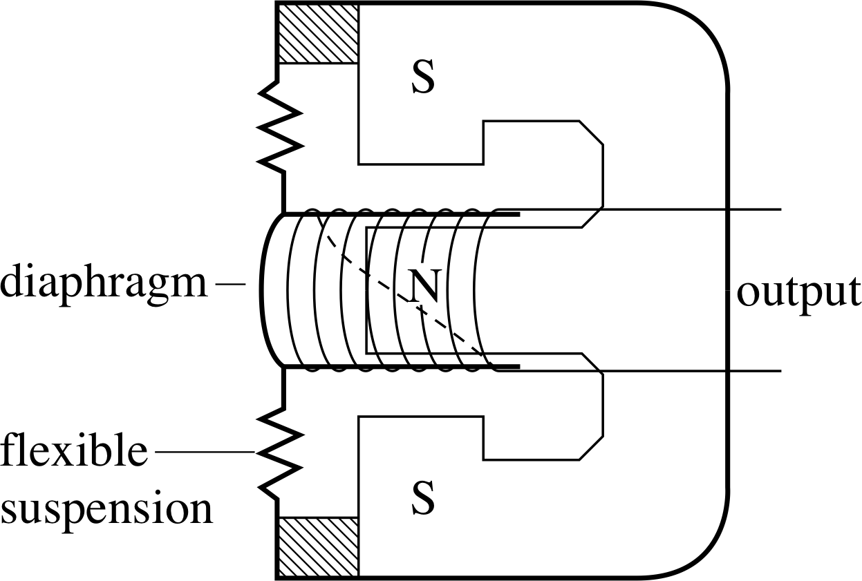
Figure 6 See Question T1.
Question T1
A microphone is a device used to produce an electrical signal from a sound signal. Figure 6 shows one type of microphone (a moving–coil microphone) which uses electromagnetic induction. i
Write one or two sentences to describe what will happen when sound waves make the diaphragm (and the attached coil) vibrate; N and S are the north and south poles of a magnet.
Answer T1
As the magnet is only half into the coil, the field around the coil is non-uniform, so when sound excites the diaphragm and causes the coil to vibrate the magnetic field within it changes, inducing a voltage. The voltage will vary according to the size and frequency of the vibrations, since both affect the speed at which the diaphragm moves.

Figure 4b The magnetic field lines around a current carrying solenoid
2.2 The polarity of an induced voltage and Lenz’s law
We can predict the polarity of an induced voltage by considering the principle of energy conservation, applied to electromagnetic induction. i Think about the situation shown in Figure 2.
Figure 2 Relative motion between a magnet and a circuit.
Suppose the bar magnet is projected towards the coil with a given speed. This motion induces a voltage and a current in the coil. The current produces a magnetic field so that the coil itself behaves as a magnet (as illustrated in Figure 4b).
✦ On energy conservation principles, would you expect the induced magnetic forces to attract or repel the approaching magnet? Would the forces differ if the magnet were moving away from the coil?
✧ We know that the induced current must represent an increase in electrical energy in the circuit since it will produce heating of the wires through which it flows. There is also energy associated with the magnetic field which results from the current. i The principle of energy conservation, applied to the system of the magnet and circuit, tells us that this gain in energy of the circuit and magnetic field must be accompanied by a reduction in kinetic energy of the moving magnet - so there must be repulsion between the coil and the magnet. If the magnet were moving away from the coil then the same argument leads to the magnet being slowed down by an attractive force.
In both these situations the induced currents flow in a direction such that the relative motion is opposed and the moving magnet is slowed down. i If you were to push the magnet into the coil or pull it out of the coil at a constant velocity then you would in each case have to work against an induced magnetic force and it is the work done by your applied force which provides the additional magnetic energy associated with the induced current.
We can express this observation also in terms of magnetic poles. If the N–pole of the bar magnet points towards the coil, then moving the magnet towards the coil must induce a current that produces another N–pole at the end of the coil which is nearest the magnet.
The argument based on energy conservation can be applied to any example of electromagnetic induction, and is generalized as Lenz’s law i:
Lenz’s law: The polarity of any induced voltage or the direction of any induced current is such as to oppose the change causing it.
Question T2
A bar magnet, with its N–pole uppermost, drops through a horizontal circular ring. Viewed from above, is the induced current clockwise or anticlockwise when (a) the S–pole of the magnet is approaching the ring, (b) the N–pole of the magnet is just leaving the ring, and (c) the magnet is half way through the ring?
Answer T2
(a) As the S–pole of the magnet approaches the ring the induced current must have a magnetic field that opposes the motion of the falling magnet. The upper side of the ring must be equivalent to a S-pole, i.e. the magnetic field of the ring must be directed downwards. The right–hand grip rule shows that the current must be clockwise when viewed from above.
(b) When the N–pole of the magnet has just passed through the ring, the magnet must be attracted towards the ring, so there must be a S–pole below the ring and the current must now be anticlockwise as viewed from above.
(c) When the magnet is halfway through the ring, Lenz’s law does not tell us what happens, but by looking at parts (a) and (b) we can guess, by continuity, that the induced current will be zero at the mid-point.
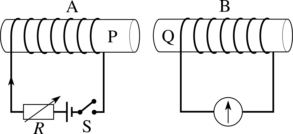
Figure 7 See Question T3.
Question T3
Use Lenz’s law to predict the directions of the current in the meter illustrated in Figure 7 when (a) switch S is closed, (b) the resistance R is then reduced, and (c) coil B is moved away from coil A with the switch closed.
Answer T3
(a) When switch S is closed, the right–hand grip rule shows that end P of the coil becomes a S-pole, with magnetic field lines directed from Q to P. Setting up this field in A induces a current in B, which produces a field in the opposite direction. End Q is therefore a S-pole, and the right–hand grip rule shows that the current must flow through the meter from left to right.
(b) If the resistance R is reduced, the current in A increases; this is an effect similar to that in (a). The field due to A increases, inducing a current in B that sets up a field in the opposite direction to oppose the change, so again the current flows from left to right through the meter.
(c) If coil B is moved away from A, the field within B due to the current in A decreases. This induces a current in B that now tries to maintain the field, i.e. the field due to the induced current is now in the same direction as that due to A, so now the current in B flows from right to left through the meter. (Instead, we could argue by forces that the current in B must induce a N–pole at Q, to produce an attractive force between the coils which will then oppose the motion.)
3 Electromagnetic induction in a complete circuit
3.1 The size of an induced voltage and Faraday’s law

Figure 8a A loop of area A in a uniform magnetic field B with the axis of the loop parallel to B.

Figure 8b A loop of area A in a uniform magnetic field B with the axis making an angle θ with B.
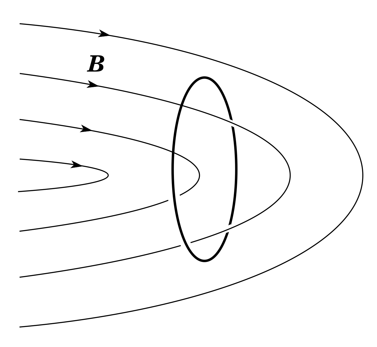
Figure 9 The net magnetic flux within this loop is zero.
In Subsection 2.1 we said, rather loosely, that electromagnetic induction occurred when there was a change in the number of magnetic field lines threading through a circuit. To make this statement a bit more precise, we need to introduce the idea of magnetic flux. Figure 8a shows a flat loop of wire, of area A, at 90° to a uniform magnetic field of magnitude B. The magnetic flux ϕ within the loop i is defined as:
ϕ = BA(2)
You can think of ϕ rather loosely as the ‘quantity of magnetic field’ enclosed by the loop. If field lines are drawn so that the number of lines crossing unit area is proportional to B, then ϕ is proportional to the number of lines within the loop. We could double the flux through a loop by doubling either the magnetic field strength or the area of the loop. i
This picture helps us to find ϕ when the loop is not ‘square-on’ to the field, as in Figure 8b. If you think of ϕ more rigorously as the product of A and the component of B at 90° to the plane of the loop, then:
The magnetic flux ϕ through a loop of area A whose axis makes an angle θ i with a uniform magnetic field B is given by
ϕ = BA cos θ(3)
Note that ϕ is a measure of the net flux through an area. If you picture magnetic field lines, only those that thread though, or ‘link’, a loop contribute to the flux through it. In Figure 9, for example, the net flux within the loop is zero – the lines entering the loop also exit from the same face and if the field lines were modelled with string, the loop could be removed without cutting them.
Note In principle ϕ can be calculated for any magnetic field crossing any surface (plane or curved). In general we would then need to break up the area into segments and add the contributions through these segments; this needs the calculus technique of integration (discussed in the maths strand of FLAP). In this module we will be concerned only with flux calculations using uniform fields crossing flat surfaces.
In SI units, B is measured in tesla (T) so from Equations 2 and 3 ϕ has SI units of T m2. However, flux is such a useful quantity that it has a unit of its own, the weber, Wb, defined so that 1 Wb = 1 T m2. i Magnetic field strength B is often called the magnetic flux density (i.e. the magnetic flux per unit area) and expressed in units of Wb m−2 (1 T = 1 Wb m−2).
Question T4
At a certain place, the Earth’s magnetic field has a strength of 48.5 μT and makes an angle of 69.6° below the horizontal. Calculate the magnetic flux within a horizontal circular loop consisting of a single turn of radius 0.50 m, at this point in the Earth’s magnetic field.
Answer T4
Flux ϕ = BA cos θ where θ is the angle between the magnetic field and the vertical, i.e. θ = 90° − 69.6° = 20.4°. Therefore
ϕ = 48.5 × 10⁻⁶ Wb m−2 × π × (0.50 m)2 × cos 20.4° = 3.57 × 10⁻⁵ Wb
In Subsection 2.1 we saw that experiments support the conclusion that the magnitude of the induced voltage in a circuit is proportional to the rate of change of magnetic field in the region around that circuit. The changing field can be produced either by changing a current or by moving a magnet.
Other experiments show that induced currents can be made to flow in a circuit even when the magnetic field does not change, provided the magnetic flux through the circuit changes. For example, in Figure 8 if the coil is rotated from its position in (a) to its position in (b) then induced currents flow in the coil, even if the magnetic field stays constant. It becomes clear then that it is the changing flux through the circuit which is the crucial factor and it is possible to identify the induced voltage as being proportional to the rate of change of magnetic flux through the circuit.
As a consequence of how the units have been defined, and the fact that 1 V = 1 Wb s−1, the constant of proportionality is unity. This result is expressed as Faraday’s law of electromagnetic induction, or simply as Faraday’s law:
Faraday’s law states that the magnitude of the induced voltage in a circuit is equal to the magnitude of the rate of change of the magnetic flux linking the circuit. i
Faraday’s law is expressed most compactly in calculus notation. For a single loop the magnitude of the voltage is given by:
Faraday’s law (single loop): $\lvert\,V_{\rm ind}\rvert = \left\lvert\,\dfrac{d\phi}{dt}\right\rvert$(4) i
Henceforth in this module in order to avoid unnecessary complication we will omit the modulus signs and leave it to you to remember that Faraday’s law only determines the magnitude of Vind. To find the polarity you must use Lenz’s law. We have so far discussed the induced voltage produced in a single loop when the flux through the loop changes. How is this modified if our ‘loop’ consists of many identical single turns, say N turns?
Experiments show that if the number of turns is increased by a factor of N, then the induced voltage is also increased by this same factor N. This should not be surprising – it simply confirms that each turn acts independently of the others and that the voltage induced overall is the algebraic sum of the individual voltages.
In modelling this situation there are two different approaches adopted by authors; these differ in how the flux linkage is defined for such a composite coil. One group leave the flux definition unchanged and write Faraday’s law as:
$V_{\rm ind} = \dfrac{d\phi}{dt}$ (magnitudes only)(5)
However, we will adopt the alternate view, which leaves Faraday’s law in the same form as in Equation 4 but redefines the total flux through the composite coil to be increased by the factor N. In this case we speak of the magnetic flux linkage Φ = Nϕ i through the composite coil as the flux per turn multiplied by the number of turns. We have:
magnetic flux linkage Φ = Nϕ (magnitudes only)(6)
and Faraday’s law then gives the magnitude of the induced voltage as:
Faraday’s law: $V_{\rm ind} = \dfrac{d{\it\Phi}}{dt}$(7) i
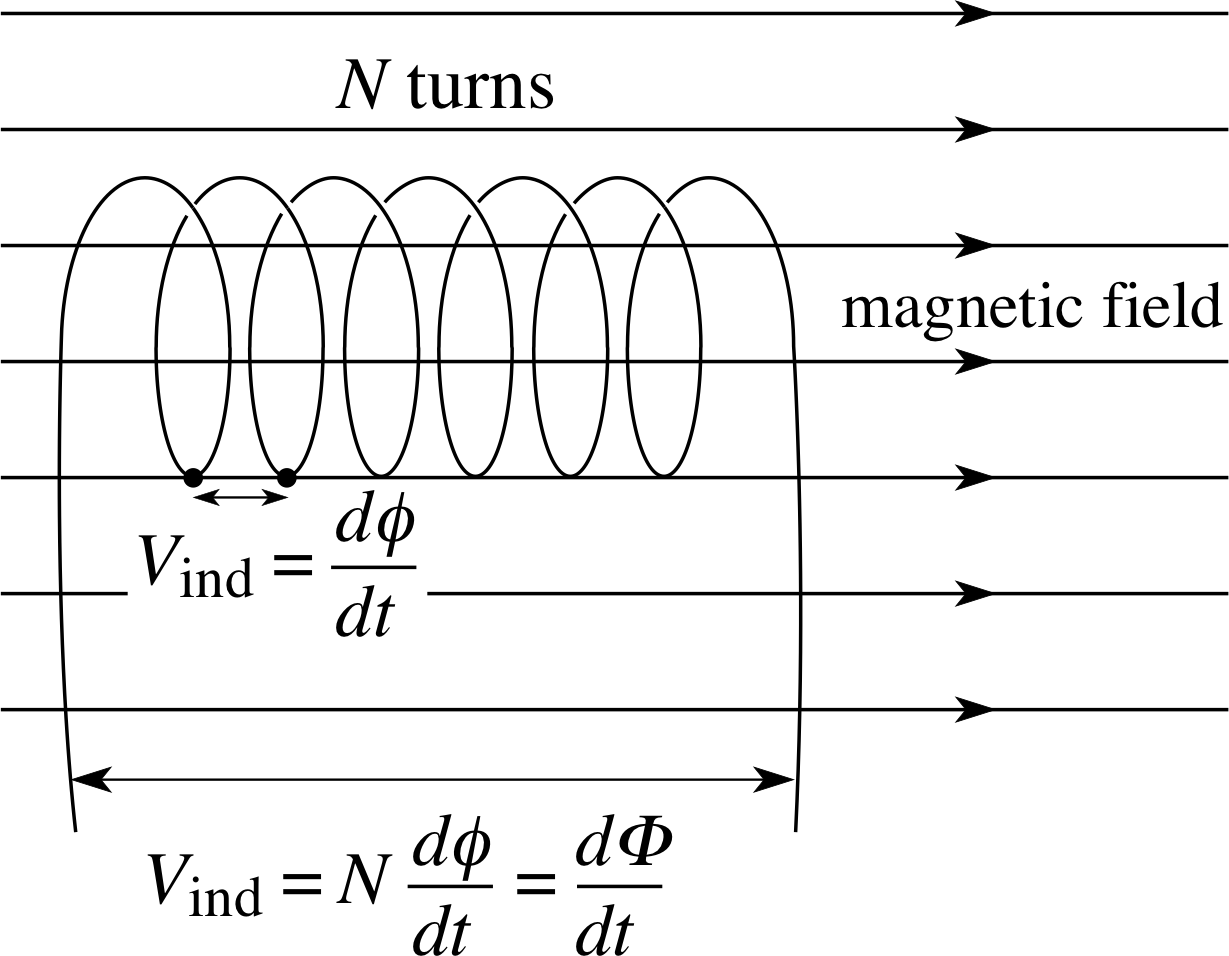
Figure 10 Each turn contributes its induced voltage to the total potential difference between the ends of a coil.
The relationships between these quantities are shown in Figure 10. Since Φ is flux multiplied by a pure number, its SI units are also Wb. However, to make its origins explicit, Φ is sometimes expressed in weber-turns. (For example, if there is a flux of 0.30 Wb within each turn of a 20 turn coil, then we can say that the flux linkage is 6.0 Wb–turns.)
Notice that Faraday’s law does not specify how the change in Φ comes about. The flux which links a circuit may change because a permanent magnet is moved near the circuit (e.g. Figures 2 and 5) or because the current in a nearby circuit changes (e.g. Figures 3 and 7), or because the circuit may move within a magnetic field (e.g. Figures 2, 6 and 7). Induction brought about by the movement of a circuit is often referred to as motional induction.
Example 1
The magnetic field strength between the poles of a strong electromagnet at a given moment is B = 0.10 T. A circular coil of radius r = 2.0 cm and having 10 turns is placed within the field and perpendicular to it. If the magnetic field strength increases steadily to 0.25 T in 1.2 ms:
(a) calculate the magnetic flux linkage in the coil initially and after 1.2 ms;
(b) calculate the voltage induced in the coil while the field is changing;
(c) If the axis of the coil had made an angle of 35° with the direction of the magnetic field, how would the induced voltage have differed?
Solution
(a) The magnetic field is perpendicular to the coil, so the initial flux per turn ϕ1 is: ϕ1 = BA = 0.10 Wb m−2 × π × (0.02 m)2 = 1.26 × 10⁻⁴ Wb and the initial flux–linkage is:
Φ1 = 1.26 × 10⁻³ Wb-turns
After 1.2 ms the final flux linkage is:
Φ2 = 0.25 Wb m−2 × π × (0.02 m)2 × 10 turns = 3.14 × 10⁻³ Wb-turns.
(b) The steady rate of change of Φ is ∆Φ/∆t = (Φ2 − Φ1)/∆t. The magnitude of the induced voltage is then:
Vind = dΦ/dt = (3.14 − 1.26) × 10−3 Wb/1.2 × 10−3 s = 1.6 V
(c) The flux per turn would be ϕ = BA cos θ, so the magnitude of the induced voltage would be Vind = 1.6 cos 35° V = 1.3 V.
Question T5
Suppose a magnetic storm causes the magnetic field of Question T4 to increase at a rate of 10.5 μT s−1, but without changing its direction. What is the magnitude of the voltage induced in the coil?
Answer T5
As only B is changing, we have dΦ/dt = A cos θ × dB/dt and so the magnitude of the induced voltage is:
Vind = π × (0.50 m)2 × cos 20.4° × 10.5 × 10⁻⁶ T s−1 = 7.73 μV
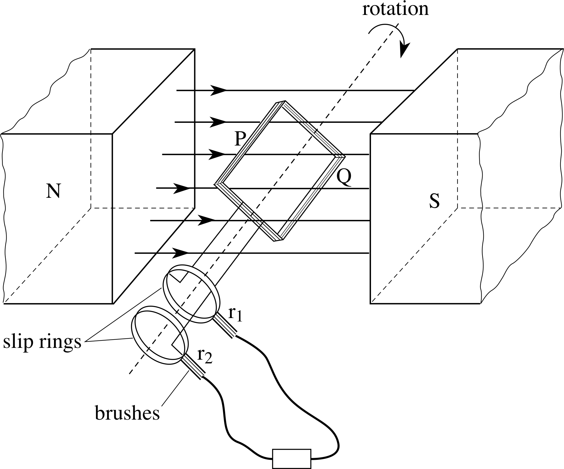
Figure 11 A simple alternator.
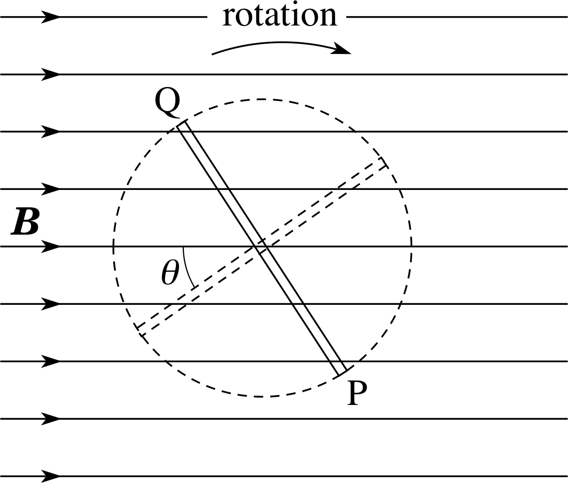
Figure 12 End–on view of the rotating alternator coil.
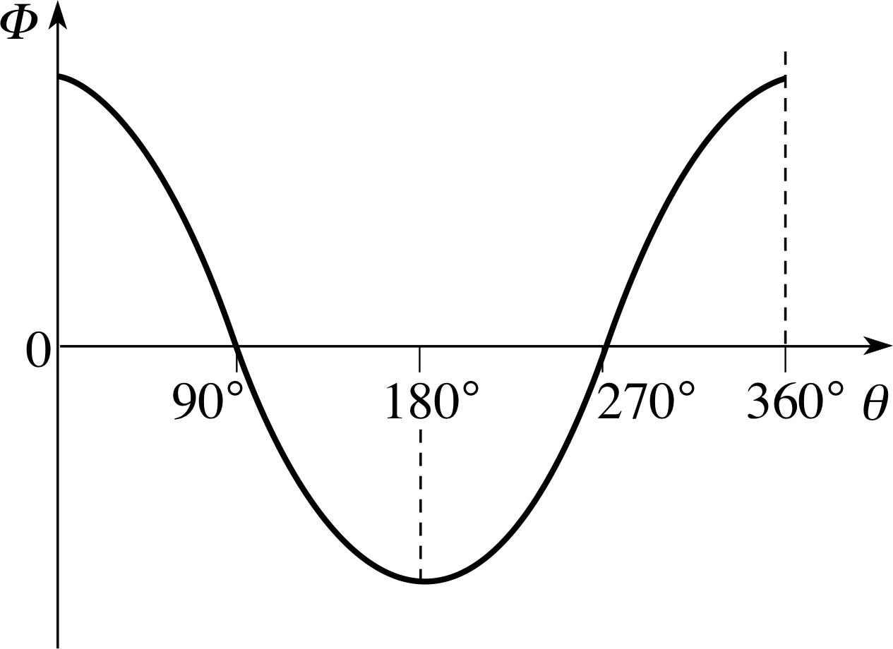
Figure 13 The flux linkage changes as the alternator coil rotates.
3.2 Alternators and dynamos
We have seen that changes in the magnetic flux linkage in a circuit gives rise to an induced voltage. If we can arrange for a continuous change in flux linkage, then we have a continuous supply of electricity – which is what happens in the generators in a power station or in a bicycle dynamo. Alternating voltages i can be generated more reliably than direct voltages, and they are easier to transform (via a transformer i) to higher or lower voltages. In a simple alternator, or a.c. dynamo, an alternating voltage is created by rotating a flat coil in a uniform magnetic field, as shown in Figure 11. i Sides P and Q of the coil are connected to the slip rings r1 and r2, which rotate with the coil and make contact with the external circuit via the two brushes.
Figure 12 shows an end–on view of the coil as it rotates, and Figure 13 shows how the flux linkage changes with angle. The flux linkage is greatest when the plane of the coil is at right angles to the field direction (θ = 0°, 180°) and zero when it is parallel to the field (θ = 90°, 270°). From Equations 3 and 6:
ϕ = BA cos θ(Eqn 3)
Φ = Nϕ(Eqn 6)
we have:
flux linkage: Φ = BAN cos θ(8)
where A is the area of each of the N turns on the coil, so Figure 13 has the shape of a cosine graph. When the coil has turned through 180° the positions of sides P and Q have been interchanged, so the direction of the flux through the coil has been reversed and we give Φ a negative sign.
From Faraday’s law,
Faraday’s law: $V_{\rm ind} = \dfrac{d{\it\Phi}}{dt}$(Eqn 7)
we can find Vind by looking at the way Φ changes with time (e.g. we could look at the slope of the graph of Φ against t). For a steady rotation, θ changes steadily with time, so a graph of Φ against t would have the same shape as a graph of Φ against θ (i.e. Figure 13). In Figure 13 we have chosen Φ positive as being for 0 < θ < 90° and 270° < θ < 360° and negative with the coil reversed, 90° < θ < 270°. The induced voltage is greatest when Φ is changing most rapidly (i.e. when the graph is steepest) and zero when the rate of change of Φ is zero. The polarity of the induced voltage depends on whether dΦ/dt (or dΦ/dθ) is positive or negative.
Question T6
Sketch a graph showing the variation of induced voltage (Vind not just | Vind |) with angle as the alternator coil rotates at a steady angular speed.
Answer T6
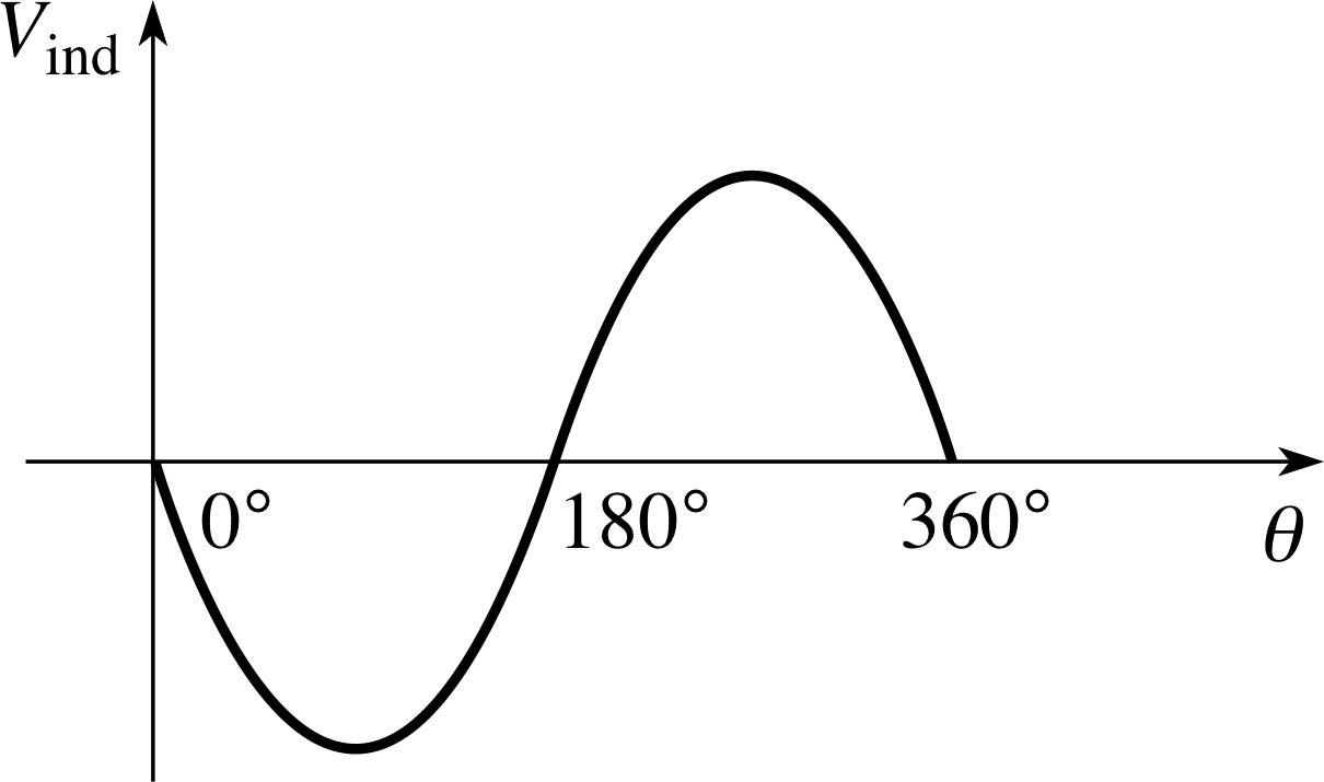
Figure 26 See Answer T6.
The graph of induced voltage against θ is given in Figure 26. The voltage is greatest when the graph in Figure 13 is steepest (e.g. when θ = 90° and 270°) and zero when Figure 13 is flat (e.g. the coil is passing through θ = 0° and 180°)
We have chosen the polarity of Vind to be negative for 0 < θ < 180° and positive for 180° < θ < 360°. The shape of this curve is seen to be a negative sine function. You could have chosen to draw this as a positive sine curve, with equal validity by adopting the opposite polarity convention.
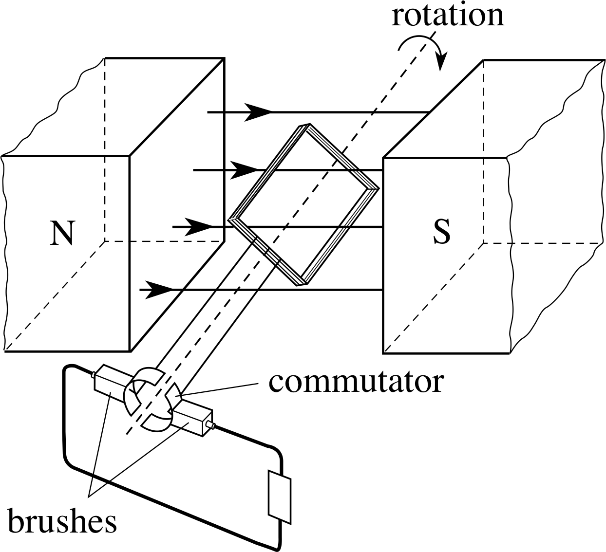
Figure 14 A simple d.c. dynamo.
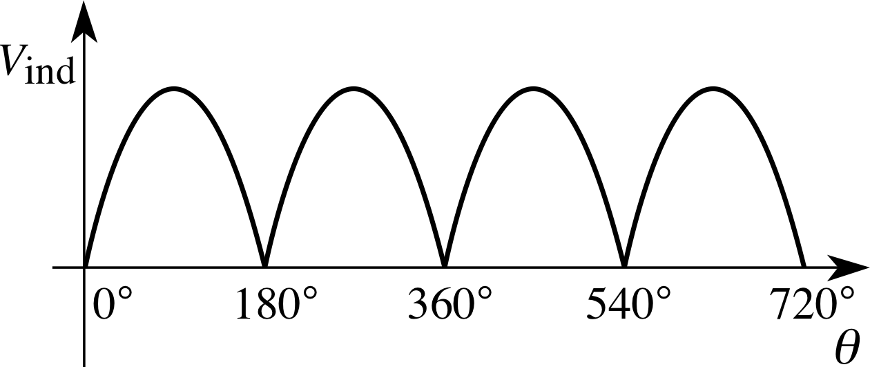
Figure 15 The output from a simple d.c. dynamo.
The output voltage is then given by Faraday’s law and Lenz’s law as (if B is constant):
$V_{\rm ind} = \dfrac{d}{dt}BAN\cos\theta = BAN\dfrac{d}{dt}(\cos\theta)$ i
Since the angular speed ω = dθ/dt this can be written as:
a.c. dynamo output $V_{\rm ind} = BAN\dfrac{d}{d\theta}(\cos\theta)\dfrac{d\theta}{dt} = -BAN\omega\sin\theta$(9)
This confirms that the induced voltage is represented by a negative sine function, as we deduced in Answer T6, since a negative sine function is the derivative of the cosine function. The absolute signs of Φ and Vind here are arbitrary.
Figure 14 shows how a simple Vind alternator can be adapted to make a d.c. dynamo. A split–ring connector is used so that, instead of side P always being connected to the same terminal of the external circuit, the connections are reversed every half cycle to give the varying d.c. output shown in Figure 15. We could write this as:
d.c. dynamo output Vind = BANω | sin θ |(10)
3.3 Measuring magnetic field strength with a search coil
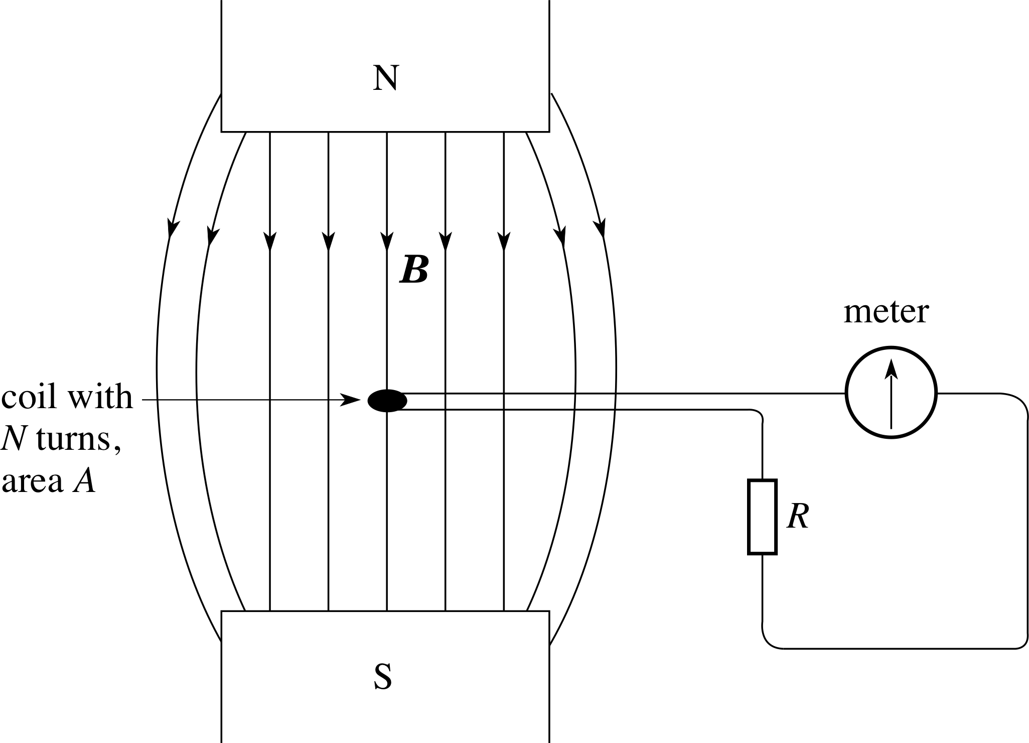
Figure 16 A search coil in a magnetic field.
We have seen that for a constant magnetic field (e.g. Equation 9 or 10), the size of an induced voltage depends on the strength of the magnetic field that produces it. In this subsection, we will see how electromagnetic induction can be exploited to measure the strength of a magnetic field. The method uses a search coil – a small flat coil, usually with many turns, which is placed in the unknown magnetic field, e.g. between the poles of a magnet, as in Figure 16.
If such a coil is quickly removed from a particular field, so that the flux linkage rapidly drops to zero, then there will be a pulse of induced current through the meter. If the coil is removed very rapidly then a relatively large current will flow for a very short time; if the coil is removed less rapidly then a relatively small current will flow for a longer time. It turns out that in each case the same total charge flows through the circuit, however the coil is removed from the field, as we will now show.
The initial flux linkage, when the coil is in the field, is found from Equation 8,
flux linkage: Φ = BAN cos θ(Eqn 8)
If the coil is then removed to a place far away from this field, then the change in flux linkage has magnitude:
∆Φ = BAN cos θ(11) i
If this change takes place in a time interval ∆t, then we can adapt Equation 7,
Faraday’s law: $V_{\rm ind} = \dfrac{d{\it\Phi}}{dt}$(Eqn 7)
to say that the average induced voltage $\langle V_{\rm ind}\rangle$ i over that time has magnitude
$\langle V_{\rm ind}\rangle = \dfrac{\Delta{\it\Phi}}{\Delta t}$
This voltage drives an average induced current $\langle V_{\rm ind}\rangle$ through the resistor R, such that
$\langle V_{\rm ind}\rangle = \dfrac{\langle V_{\rm ind}\rangle}{R} = \dfrac{\Delta{\it\Phi}}{R\Delta t}$
The total charge that flows, ∆q, is given by:
$\Delta q = \langle V_{\rm ind}\rangle\Delta t = \dfrac{\Delta{\it\Phi}}{R} = \dfrac{BAN}{R}\cos(\theta)$(12)
This total flow of charge is proportional to the initial flux linkage and therefore to the magnetic field strength, irrespective of the speed of removal of the search coil. After suitable calibration i this produces a means of measuring magnetic field strength. The coil is usually inserted perpendicular to the magnetic field (θ = 90°) and then removed from the field, to give a charge flow which is proportional to the initial field. Thus, by measuring the charge flow and knowing the geometry of the search coil, we can measure the component of magnetic field at right angles to the plane of the coil. i
There are two instruments in common use to measure these charge flows. Both of these are based on the principle of the moving–coil galvanometer (MCG). i The first instrument, called a ballistic galvanometer, has a coil mounted on a very weak suspension. A current pulse through the coil produces an impulse on the coil which results in an initial swing, the amplitude of which is proportional to the charge flowing in the current pulse.
The second instrument, called a fluxmeter, has no restoring couple on the suspension but only a damping resistive force. In this case the current pulse produces a non–returning deflection of the coil, the size of which is determined by the total charge flowing and the damping of the suspension. The fluxmeter must also have the facility to restore the coil to its central position (re-zeroing) by injecting a current pulse from some internal supply. Both instruments give a deflection which is proportional to the flux change in the search coil and so can be calibrated to allow the measurement of the initial field within this coil. The fluxmeter is slightly easier to use since, when the instrument is carefully levelled, its deflection is non–returning and hence easier to record.
Question T7
A search coil with area 2.0 cm2 and 50 turns is attached to a ballistic galvanometer and is placed with its plane at right angles to the field between the poles of a magnet. The total circuit resistance is 200 Ω. When the coil is suddenly removed from the field the meter measures a total charge flow of 2.4 μC. Calculate the field strength of the magnet.
Answer T7
Using Equation 12,
$\Delta q = \langle V_{\rm ind}\rangle\Delta t = \dfrac{\Delta{\it\Phi}}{R} = \dfrac{BAN}{R}\cos(\theta)$(Eqn 12)
with cos θ = 1, gives
B = R∆q/AN = 200 Ω × 2.4 × 10−6 C/(2.0 × 10−4 m2 × 50) = 0.05 T
Question T8
How much charge flows through the meter in Question T7 if, instead of being removed from the field, the search coil is quickly flipped over through 180°?
Figure 11 A simple alternator.
Answer T8
The situation is similar to that in the alternator (Figures 11 and 13).
Figure 13 The flux linkage changes as the alternator coil rotates.
If the initial flux linkage is Φ, then the flux linkage after flipping the coil is −Φ.
The magnitude of ∆Φ is therefore 2Φ, and so twice as much charge flows as before, i.e. 4.8 μC.
4 Transformers
When two circuits are in close proximity, any change in the current in one will induce currents in the other, and vice-versa. Such circuits are said to be magnetically coupled. This coupling can be very useful and in some applications it is an important design criterion to maximize the proportion of the magnetic field lines produced by each circuit which link through the other circuit – to optimize the flux linkage. To achieve this the circuits are often coils and the coils are wound on a common iron core. Iron has a high relative permeability i and this has the effect of providing a preferred route through the iron for the magnetic field lines, channelling the magnetic field lines so that almost all lines produced by one coil also pass through the other coil, with little or no magnetic flux leakage. Such devices are called transformers and they find widespread application.
4.1 Transformers
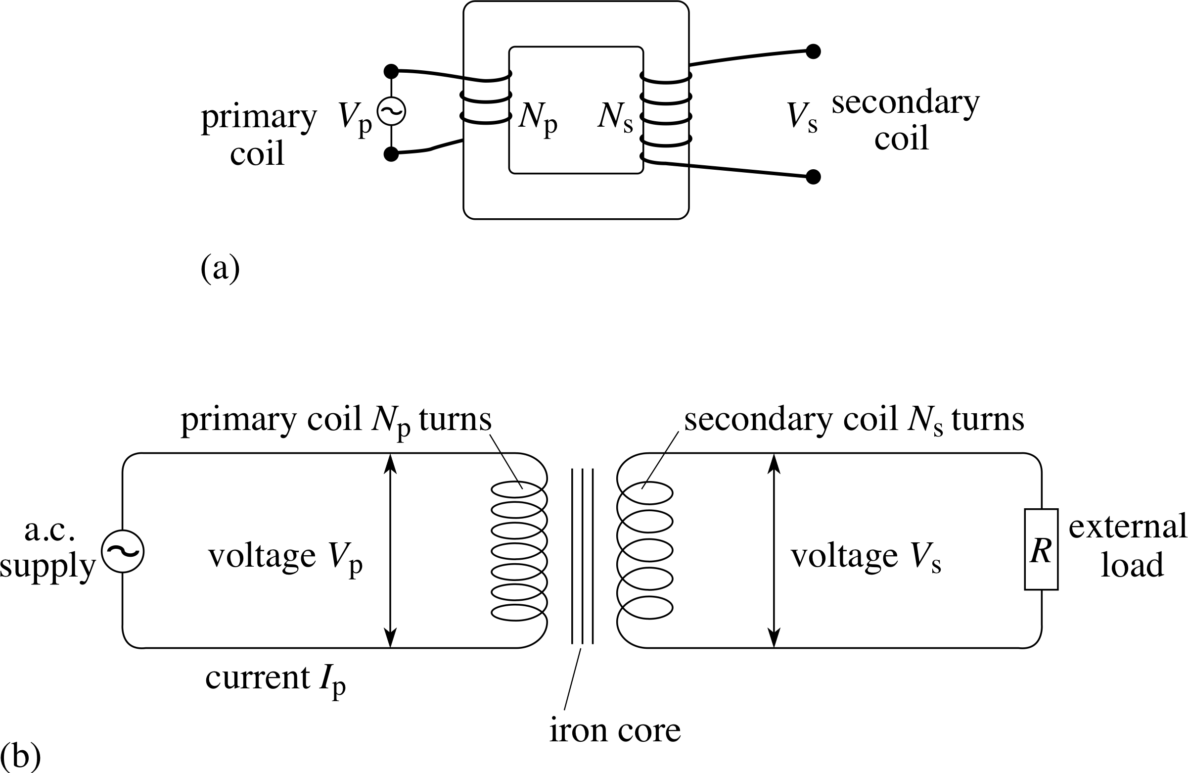
Figure 17 A transformer. (a) One possible physical arrangement, (b) schematic representation of the circuit.
In Subsection 3.2 we said that a.c. voltages were easy to transform to higher or lower voltages. This is the main function of a transformer, such as is illustrated in Figure 17. i The two coils are wound on a common iron core, either one on top of the other or occupying separate parts of the core as in Figure 17a.
Figure 17b shows the circuit symbol for a transformer. The primary coil is connected across the input power supply and the secondary coil is connected to an external circuit. Since the primary current is alternating, the flux within the core varies continuously and the changing flux linkage in the secondary coil induces an a.c. voltage and current in the secondary circuit. For a given primary voltage, transformers can be used to produce a wide range of secondary voltages. If there is no flux loss, each magnetic field line generated by the primary circuit links each turn in the primary and secondary circuits. We deduce that the same flux per turn links the primary and the secondary coils, so ϕp = ϕs. The situation of no flux leakage is one requirement of what is called an ideal transformer. In this case, the total flux linkage in the primary and secondary coils is in the ratio of the numbers of turns on these two coils:
$\dfrac{\Delta{\it\Phi}_{\rm s}}{\Delta{\it\Phi}_{\rm p}} = \dfrac{N_{\rm s}\Delta\phi_{\rm s}}{N_{\rm p}\Delta\phi_{\rm p}} = \dfrac{N_{\rm s}}{N_{\rm p}}$(13)
Since the induced voltages in the primary and secondary are in the ratio of the rate of change of total flux linkage in these two coils, we have:
For an ideal transformer: $\dfrac{V_{\rm s}}{V_{\rm p}} = \dfrac{d{\it\Phi}_{\rm s}/dt}{d{\it\Phi}_{\rm p}/dt} = \dfrac{N_{\rm s}(d\phi_{\rm s}/dt)}{N_{\rm p}(d\phi_{\rm p}/dt)} = \dfrac{N_{\rm s}}{N_{\rm p}}$(14) i
Equation 14 expresses the transformer voltage ratio in terms of the turns ratio, Ns/Np; for a given primary voltage and primary coil, the secondary voltage can be controlled by the number of turns on the secondary coil.
✦ For a given magnetic flux density B, what happens to the flux linkage Φs in the secondary coil if you change the number of turns Ns? As a consequence, what happens to the secondary voltage Vs?
✧ Increasing Ns increases Φs. For a given B, this increases Vs. Since Φs ∝ Ns, and Vs ∝ dΦs/dt ∝ Ns, then Vs ∝ Ns.
Equation 14 tells us that we can, in principle, design a transformer to increase an a.c. voltage by any desired amount (step–up transformer) or reduce it by any desired amount (step–down transformer) – simply by using coils with suitable numbers of turns.
A step–up transformer in which the output secondary voltage exceeds the input primary voltage, might appear to be giving us something for nothing. However, energy conservation tells us that this is not the case. The output power from the secondary is provided by the input power to the primary. Another characteristic of an ideal transformer is that there is no power transformed into other forms, such as heat or sound. i
We can thus define an ideal transformer as one in which the flux linkage is complete and electrical power is transformed with 100% efficiency. In this case, if the transformer is ideal then these two powers would be equal, so that:
IpVp = IsVs(15)
and Ip/Is = Vs/Vp = Ns/Np(16)
Equation 16 tells us that if the secondary voltage exceeds the primary voltage then the secondary current must be less than the primary current. In this way a transformer can also be used to transform the currents between two circuits as well as the voltages between them.
In practice, there are several reasons why no transformer is ideal. First, the coils have d.c. resistance and so there is always some power transferred into heating of the coils within the transformer. Also, the continuous variations in magnetic field mean that sections of the core repeatedly attract and release each other, giving rise to an audible chatter or hum – which produces sound energy. You may have noticed the characteristic 100 Hz hum of mains transformers – the mains frequency is 50 Hz so the field reaches a peak magnitude 100 times per second. There is another process, called eddy current generation in the core itself, (we will discuss this in Subsection 5.3) which produces heating. Despite these processes, most transformers can transfer over 80% of the energy from the primary to the secondary circuit.
Another use of a transformer is to allow two circuits to communicate through the magnetic coupling whilst they remain electrically isolated from each other. For example, an a.c. signal applied to the primary circuit gives an a.c. signal on the secondary without the two coils being electrically connected. This finds application where the two coils must be at very different d.c. voltages – such as with the signal applied to a television picture tube, where the latter is at an electrical potential which is several tens of kV different from ground potential. For safety reasons the two parts of the circuit must be kept electrically isolated. This use of a transformer is called d.c. isolation.
This same feature of d.c. electrical isolation with a.c. magnetic coupling is also used where the a.c. signal must be transferred from one circuit to another but where the electrical resistances or impedances i are very different in the two circuits. For example, the input to an amplifier might require quite a high input impedance but the microphone to be connected to it is often part of a low impedance circuit. The two may be connected through a transformer with the primary (microphone side) having low impedance and the secondary (amplifier side) having a high impedance. This use of a transformer is called impedance matching.
Question T9
A bathroom shaver socket is labelled 110 V. Behind the socket is an ideal transformer with a 500 turn primary coil connected to the 240 V mains. (a) How many turns must there be in the secondary coil? (b) Calculate the secondary and primary currents when a 10 W shaver is connected to the socket.
Answer T9
(a) Using Equation 14:
$\dfrac{V_{\rm s}}{V_{\rm p}} = \dfrac{N_{\rm s}}{N_{\rm p}}$(Eqn 14)
Ns = Np × Vs/Vp = 500 × 110 V/240 V = 229 (to the nearest whole number)
(b) Since secondary and primary powers are equal for an ideal transformer,
Ps = IsVs = IpVp = Pp
soIs = Ps/Vs = 10 W/110 V = 0.091 A = 91 mA
and Ip = 10 W/240 V = 0.042 A = 42 mA
Alternatively, from Equation 16,
Ip/Is = Vs/Vp = Ns/Np(Eqn 16)
Ip = Is × Ns/Np = 91 mA × 229/500 = 42 mA
4.2 Mutual inductance and self inductance
In the previous subsection we treated the primary coil as the source of the alternating current and the secondary coil as responding to the primary through induction. There are two problems with this simple view.
First, the current fluctuations in the secondary coil also cause magnetic flux changes in the primary and hence induced currents flow in the primary in response to the secondary currents. We might say that the secondary coil reacts back on the primary coil and so the distinction between a primary coil and a secondary coil is rather artificial. It is more realistic to think of the two coils as being mutually coupled – the changes in either coil affecting the other coil in a process called mutual induction. We say that the two coils together have mutual inductance.
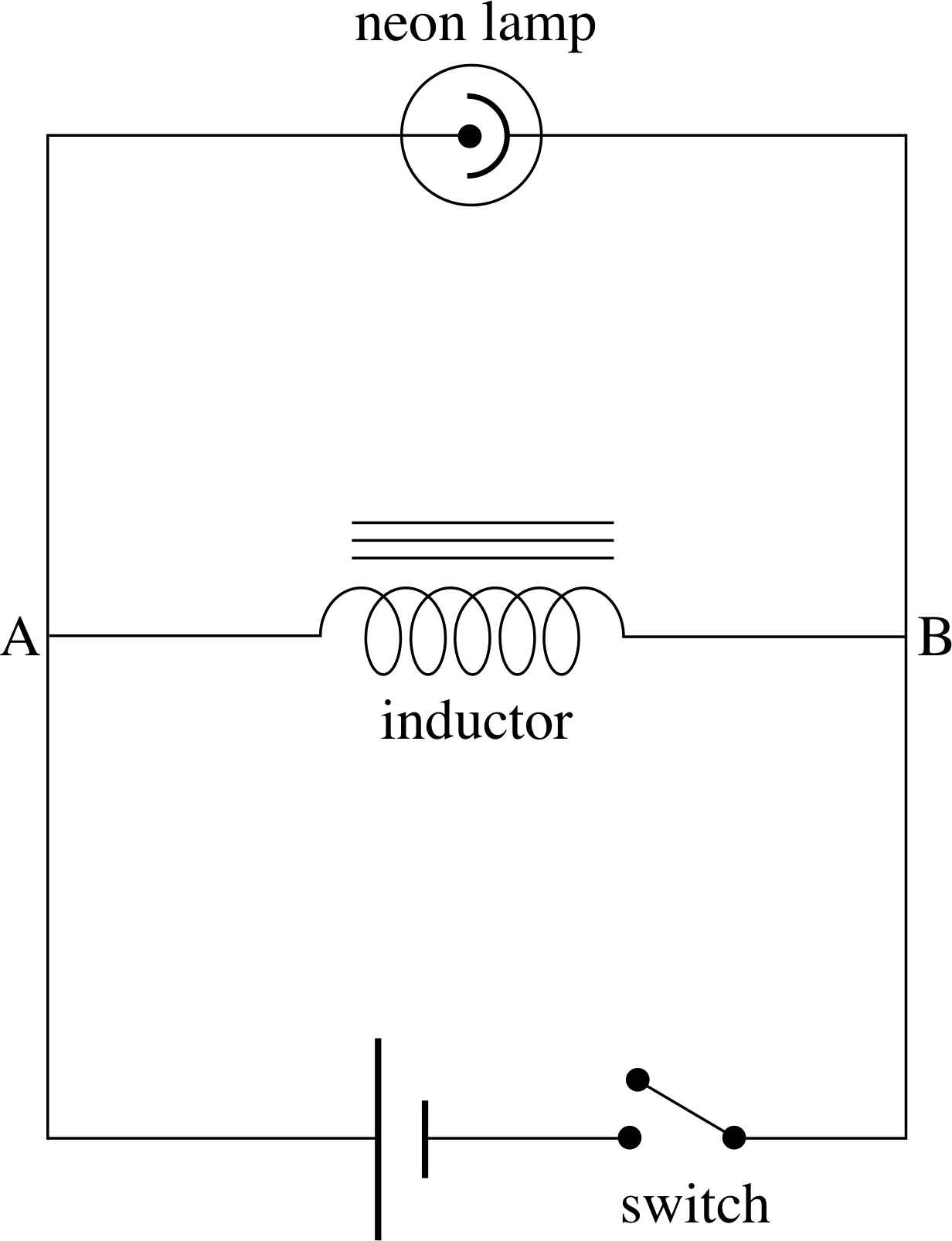
Figure 18 Circuit to demonstrate self induction.
The second problem is that even with a single coil the current fluctuations give rise to fluctuating magnetic fields around the coil itself and these produce flux changes and induced currents in the same coil. If we attempt to change the current in a coil we find that the coil produces an induced voltage between its ends and by Lenz’s law the direction of this induced voltage is such as to resist the change of current. This process is called self induction and the coil is said to have self inductance. Any coil, or indeed any wire, has some self inductance, but to produce appreciable self inductance it is usually necessary to have many nearby turns on the coil or to wind the coil on a core of material with a high relative permeability. A coil with appreciable self inductance is called an inductor.
Self-induction may be demonstrated using the circuit shown in Figure 18. i A neon bulb will conduct only when the voltage across it exceeds about 80 V, at which point ionization occurs within the gas, there is a rapid movement of ions and electrons and the excited gas glows; at lower voltages its resistance is effectively infinite. With the switch closed and a steady current established in the inductor, the neon lamp does not glow. When the switch is opened, the current in the coil rapidly falls to zero and the induced voltage in the coil exceeds the 80 V and the lamp flashes briefly. The same happens as the switch is first closed. The iron core and the large number of turns ensure that even a small current produces a large flux linkage in the coil.
Aside The induction coil on a car ignition system is another example of a device which uses induction produced by interrupting the current in a circuit. In this case two coils are used, as in a conventional step–up transformer, but the induced voltage produced in the secondary coil arises when the current in the primary coil is rapidly interrupted. Here the primary circuit consists of a d.c. current provided by the 12 V car battery and when this circuit is periodically interrupted by a rotating contact breaker there are voltage pulses of several tens of kV, which produce the sparks to ignite the fuel.
✦ In Figure 18, what can you deduce about the direction of the induced voltage and the induced current when the switch is opened?
✧ Before the switch is opened, the current in the coil flows from A to B. Lenz’s law tells us that the induced voltage opposes the change that causes it. The self induced voltage must therefore be ‘trying’ to maintain the magnetic flux within the coil by continuing to drive current through the coil from A to B (i.e. anticlockwise around the top loop of the circuit). Since the self induced voltage always opposes the change that is causing it, it is sometimes called a back voltage.
We need to characterize the self inductance of a coil in some way. Faraday’s law, Equation 7, gives the magnitude of the induced voltage as:
$V_{\rm ind} = \dfrac{d{\it\Phi}}{dt}$ (magnitudes only)(Eqn 7)
We also know that the magnetic field around a coil and hence the flux linkage Φ is proportional to the coil current I. We can therefore say that, for a given coil, the magnitude of the self induced voltage is proportional to the rate of change of current. The constant of proportionality is called the coefficient of self inductance (often just the inductance) of the coil and is given the symbol L, which is defined by Φ = LI.
The magnitude of the voltage across the inductor, VL, is then given by:
inductor voltage magnitude $V_{\rm ind} = V_L = L\,\left\lvert\,\dfrac{dI}{dt}\,\right\rvert$(17) i
L has SI units of V s A−1, but this has been named the henry, H, where 1 H = 1 V s A−1. i
We will end this subsection by deriving an expression for the inductance of a long solenoid – N turns of area A in a length l. If this coil carries a current I, the magnetic field inside the coil has magnitude:
solenoid field with air core: $B = \dfrac{\mu_0NI}{l}$(18) i
If the coil is wound on a core of relative permeability μr then the field is increased by the factor μr to become:
solenoid field with magnetic core: $B = \dfrac{\mu_{\rm r}\mu_0NI}{l}$(19)
From Equations 3 and 6,
ϕ = BA cos θ(Eqn 3)
magnetic flux linkage: Φ = Nϕ(Eqn 6)
the flux linkage Φ is therefore
${\it\Phi} = BAN = \dfrac{\mu_{\rm r}\mu_0AN^2I}{l}$(20)
Faraday’s law (Equation 7)
$V_{\rm ind} = \dfrac{d{\it\Phi}}{dt}$ (magnitudes only)(Eqn 7)
then gives the magnitude of the induced voltage:
$V_L = \left\lvert\,\dfrac{d{\it\Phi}}{dt}\,\right\rvert = \left\lvert\,\dfrac{d}{dt}\left(\dfrac{\mu_{\rm r}\mu_0AN^2}{l}\right)\,\right\rvert = \dfrac{\mu_{\rm r}\mu_0AN^2}{l}\left\lvert\,\dfrac{dI}{dt}\,\right\rvert = L\,\left\lvert\,\dfrac{dI}{dt}\,\right\rvert$(21)
From which it is apparent that for this solenoid:
$L = \dfrac{\mu_{\rm r}\mu_0AN^2}{l}$(22) i
So, the inductance of a coil of fixed length is proportional to the square of the number of turns, assuming it may be treated as a long solenoid. i
Question T10
A long solenoid has 4000 turns wound on a cylinder of magnetic material with μr = 1700, with radius 0.80 cm and length 7.0 cm. (a) Calculate the inductance of the coil. (b) If the current in the coil increases at the rate of 0.753 A s−1 find the induced voltage.
Answer T10
(a) From Equation 22,
$L = \dfrac{\mu_{\rm r}\mu_0AN^2}{l}$(Eqn 22)
the inductance is:
L = 1700 × 4π × 10−7 H m−1 × π × (0.80 × 10⁻² m)2 × (4000)2/0.070 m = 98 H (= 98 V s A−1)
This inductor would be quite heavy and we see that the henry is a large unit of inductance!
(b) From Equation 21,
$V_L = \left\lvert\,\dfrac{d{\it\Phi}}{dt}\,\right\rvert = \left\lvert\,\dfrac{d}{dt}\left(\dfrac{\mu_{\rm r}\mu_0AN^2}{l}\right)\,\right\rvert = \dfrac{\mu_{\rm r}\mu_0AN^2}{l}\left\lvert\,\dfrac{dI}{dt}\,\right\rvert = L\,\left\lvert\,\dfrac{dI}{dt}\,\right\rvert$(Eqn 21)
the self induced voltage has magnitude:
$V_L = L\,\left\lvert\,\dfrac{dI}{dt}\,\right\rvert = \rm 98\,V\,s\,A^{-1}\times0.753\,A\,s^{-1}= 74\,V$
If we now return to the situation of mutual inductance between two coils, we can follow a similar path and define a coefficient of mutual inductance by relating the voltage induced in one coil to the rate of change of current in the other coil. For the primary and secondary coils of a transformer we have the magnitudes of these induced voltages given by:
induced secondary voltage $V_{\rm s} = M_{\rm sp}\left\vert\,\dfrac{dI_{\rm p}}{dt}\,\right\rvert$(23a)
induced primary voltage $V_{\rm p} = M_{\rm ps}\left\vert\,\dfrac{dI_{\rm s}}{dt}\,\right\rvert$(23b)
where Msp is the coefficient of mutual inductance relating induced secondary voltage to current changes in the primary, and Mps is the coefficient of mutual inductance relating induced primary voltage to current changes in the secondary. These two coefficients need not be equal, as we will see.
4.3 Self inductance and mutual inductance in a transformer
We now apply the work of the previous subsection to an ideal transformer. The primary current generates a magnetic field in the core and this field is also conveyed to the secondary coil through the core. Changes in the primary current cause induced secondary currents and these also contribute to the field in the core. By Lenz’s law the secondary currents must produce fields in opposition to the changes in the primary field contribution. Though the field contributions themselves must be added or subtracted depending on the changes in B.
solenoid field with magnetic core: $B = \dfrac{\mu_{\rm r}\mu_0NI}{l}$(Eqn 19)
we can write the magnitude of the total field in the core as:
$B = \dfrac{\mu_{\rm r}\mu_0N_{\rm p}I_{\rm p}}{l_{\rm p}} \pm \dfrac{\mu_{\rm r}\mu_0N_{\rm s}I_{\rm s}}{l_{\rm s}}$(24)
where the subscripts identify the coil concerned.
The flux in the two coils is then given by Equation 8,
flux linkage: Φ = BAN cos θ(Eqn 8)
as:${\it\Phi}_{\rm p} = BAN_{\rm p} = \mu_{\rm p}\mu_0A\left(\dfrac{N_{\rm p}^2I_{\rm p}}{l_{\rm p}}\pm\dfrac{N_{\rm p}N_{\rm s}I_{\rm s}}{l_{\rm s}}\right)$(25)
${\it\Phi}_{\rm s} = BAN_{\rm s} = \mu_{\rm p}\mu_0A\left(\dfrac{N_{\rm p}N_{\rm s}I_{\rm p}}{l_{\rm p}}\pm\dfrac{N_{\rm s}^2I_{\rm s}}{l_{\rm s}}\right)$(26)
Equation 7,
$V_{\rm ind} = \dfrac{d{\it\Phi}}{dt}$(Eqn 7)
gives the magnitudes of the induced voltage on the two coils as:
$V_{\rm p} = \left\lvert\,\dfrac{d{\it\Phi}_{\rm p}}{dt}\,\right\rvert = AN_{\rm p}\left\lvert\,\dfrac{dB}{dt}\,\right\rvert = \mu_{\rm p}\mu_0A\left\lvert\,\dfrac{N_{\rm p}^2}{l_{\rm p}}\dfrac{dI_{\rm p}}{dt}\pm\dfrac{N_{\rm p}N_{\rm s}}{l_{\rm s}}\dfrac{dI_{\rm s}}{dt}\,\right\rvert = \left\lvert\,L_{\rm p}\dfrac{dI_{\rm p}}{dt}\pm M_{\rm ps}\dfrac{dI_{\rm s}}{dt}\,\right\rvert$(27)
$V_{\rm s} = \left\lvert\,\dfrac{d{\it\Phi}_{\rm s}}{dt}\,\right\rvert = AN_{\rm s}\left\lvert\,\dfrac{dB}{dt}\,\right\rvert = \mu_{\rm p}\mu_0A\left\lvert\,\pm\dfrac{N_{\rm p}N_{\rm s}}{l_{\rm p}}\dfrac{dI_{\rm p}}{dt}+\dfrac{N_{\rm s}^2}{l_{\rm s}}\dfrac{dI_{\rm s}}{dt}\,\right\rvert = \left\lvert\,\pm M_{\rm sp}\dfrac{dI_{\rm p}}{dt}+L_{\rm s}\dfrac{dI_{\rm s}}{dt}\,\right\rvert$(28)
From these expressions we can compare coefficients and identify that:
primary self inductance$L_{\rm p} = \dfrac{\mu_{\rm r}\mu_0AN_{\rm p}^2}{l_{\rm p}}$(29)
secondary self inductance$L_{\rm s} = \dfrac{\mu_{\rm r}\mu_0AN_{\rm s}^2}{l_{\rm s}}$(30)
P–S mutual inductance$M_{\rm ps} = \dfrac{\mu_{\rm r}\mu_0AN_{\rm p}N_{\rm s}}{l_{\rm s}}$(31)
S–P mutual inductance$M_{\rm sp} = \dfrac{\mu_{\rm r}\mu_0AN_{\rm p}N_{\rm s}}{l_{\rm p}}$(32)
Equations 27 and 28 confirm the result (Equation 13) that: Vs/Vp = Ns/Np
Question T11
For the pair of coils discussed above, show that Vs/Vp = Msp/Lp = Ls/Mps, so that LpLs = MpsMsp.
Answer T11
Msp, Mps, Lp and Ls all share a common factor μ0μrA. From Equations 29 to 32,
primary self inductance$L_{\rm p} = \dfrac{\mu_{\rm r}\mu_0AN_{\rm p}^2}{l_{\rm p}}$(29)
secondary self inductance$L_{\rm s} = \dfrac{\mu_{\rm r}\mu_0AN_{\rm s}^2}{l_{\rm s}}$(30)
P–S mutual inductance$M_{\rm ps} = \dfrac{\mu_{\rm r}\mu_0AN_{\rm p}N_{\rm s}}{l_{\rm s}}$(31)
S–P mutual inductance$M_{\rm sp} = \dfrac{\mu_{\rm r}\mu_0AN_{\rm p}N_{\rm s}}{l_{\rm p}}$(32)
$\dfrac{M_{\rm sp}}{L_{\rm p}} = \dfrac{N_{\rm s}}{N_{\rm p}} = \dfrac{V_{\rm s}}{V_{\rm p}} \quad\text{and} \quad\dfrac{L_{\rm s}}{M_{\rm ps}} = \dfrac{N_{\rm s}}{N_{\rm p}} = \dfrac{V_{\rm s}}{V_{\rm p}}$
so thatLpLs = MpsMsp, as expected.
5 Motional electromagnetic induction in a single conductor
The total electromagnetic force on a charged particle, arising from the combined electric and magnetic forces, is known as the Lorentz force and it is expressed in the Lorentz force law:
Lorentz force law: F = q (E + υ × B)(33)
where the electric field is E, the magnetic field is B and the velocity of the charge is υ.
In this module we have been describing electromagnetic induction in terms of Faraday’s law, without reference to the Lorentz force. If charges are to begin to flow as induced currents then, presumably, forces must be acting on these charges to cause this motion. So, there must be some relationship between Faraday’s law and the Lorentz force. In this section we will explore this relationship and then go on to consider motional electromagnetic induction in more detail.
5.1 Faraday’s law and the Lorentz force
Study comment For simplicity, in this subsection we will deal only with a straight wire moving at right angles both to its own length and to the field direction, but the analysis could be extended, using vectors, to other orientations.
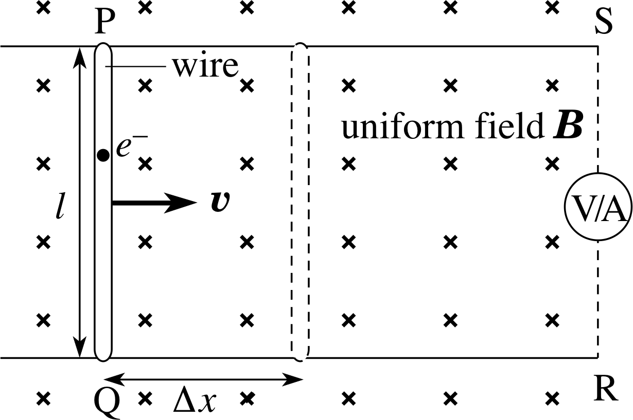
Figure 19 A wire PQ moving at right angles to a magnetic field.
Consider the situation shown in Figure 19. The straight wire PQ is moving at constant velocity at right angles to a uniform magnetic field, directed into the plane of the page. Wires PS and QR are fixed and continue to make contact with the moving wire. As PQ moves to the right, the flux linkage in the circuit SPQR reduces since the area reduces and a voltage is induced between S and R. A voltmeter may be connected between S and R and this then measures the open circuit voltage induced between the ends of the moving wire, but does not allow current to flow around the circuit. Alternatively, the voltmeter may be replaced by an ammeter, which allows induced current to flow around the circuit.
According to Faraday’s law, the flux change in this circuit will induce a voltage in the circuit and this voltage must be equated to that across PQ, as this is the only moving part of the circuit. With the voltmeter in place the voltage will be measured directly; with the ammeter inserted, the induced currents will flow, driven by the induced voltage across PQ. The question we now ask is how does this voltage arise according to the Lorentz force?
In the wire PQ there are some electrons which are free to move through the wire in response to any force acting on them (i.e. free electrons). The Lorentz force is one such force, caused by the motion of the e− electrons through the magnetic field, as they are carried along with the wire. This force is given by Equation 33, i
Lorentz force law: F = q (E + υ × B)(Eqn 33)
The direction of the force on the electrons (q = −e) is in the direction
−(υ × B), or towards Q, and its magnitude is:
F = eυB(34)
This force causes free electrons in PQ to move towards Q, or conventional current to flow from Q to P. For the conventional current direction:
The direction of the induced current flow when a conductor moves with velocity υ through a magnetic field B is the direction of the force on an assumed positive charge and so is the direction of the vector (υ × B).
✦ In the situation where currents cannot flow around the circuit, what prevents all the free electrons in PQ moving to Q?
✧ As more and more electrons are pushed to Q a net negative charge would build up at Q, with a net positive charge at P. The increasing negative charge at Q will tend to repel further electron flow. Alternatively, we can say that as the charge separation develops, an electric field in the wire will grow in the direction PQ.
This electric field will oppose further electron motion towards Q. As the electric field grows it will eventually reach a steady state situation in which the electric force on an electron will be equal and opposite to the magnetic force and so no further charge separation will occur.
In this situation the total Lorentz force on a charge in the wire is zero and Equation 33 then gives:
E + υ × B = 0
so the magnitude of the steady state electric field in the wire is: E = υB
and the voltage across the wire of length l is:
Vind = El = υBl(35)
We can compare this with the magnitude of the voltage induced in the circuit according to Faraday’s law (Equation 7):
$V_{\rm ind} = \dfrac{d{\it\Phi}}{dt}$ (magnitudes only)(Eqn 7)
The flux linkage in circuit SPQR is given by Equation 8,
flux linkage: Φ = BAN cos θ(Eqn 8)
as: Φ = BA
If the wire moves a distance ∆x in a time ∆t the flux change is ∆Φ = B∆A with ∆A = l∆x and so the magnitude of the induced voltage across PQ is:
$V_{\rm ind} = B\dfrac{\Delta A}{\Delta t}= Bl\dfrac{\Delta x}{\Delta t} = \upsilon Bl$ (magnitudes only)(36)
which is in agreement with Equation 35,
Vind = El = υBl(Eqn 35)
the result obtained from the Lorentz force law. The polarity of this voltage and the direction of the induced current flow can be found from Lenz’s law, applied either in terms of the flux changes in the circuit or the forces on PQ.
Suppose the circuit is completed by the ammeter and current is allowed to flow around the circuit. It must flow in a direction to try to maintain the flux linkage through the circuit as the circuit area is being reduced e− by the motion of PQ. This means that it must produce an additional magnetic field downwards through the circuit of Figure 19 and this requires positive current to flow clockwise around PSRQ – this is consistent with electrons flowing in the direction PQ, as we have deduced. i Lenz’s law will also predict that the induced current will produce a force on PQ which is in a direction opposing the motion of PQ. Equation 33,
Lorentz force law: F = q (E + υ × B)(Eqn 33)
shows that to give a force opposite to υ requires positive current to flow from Q to P, as we have already deduced.
Aside We see that for motional electromagnetic induction the application of the Lorentz force law allows us to predict both the magnitude and direction of flow of induced currents and in this situation is equivalent to the information provided by both Faraday’s law and Lenz’s law. Remember that Faraday’s law is also able to account for induction where flux changes take place without the motion of a conductor, such as where B is changing around a fixed circuit – the Lorentz force law has nothing to say about this situation. It is also true that Lenz’s law often provides a quick, convenient method of predicting the direction of induced currents, even in quite complicated situations. Advanced treatments of electromagnetism absorb Faraday’s law and Lenz’s law into a more powerful set of statements, called Maxwell’s equations of electromagnetism, as we mentioned in Subsection 2.1, but this is beyond the scope of this module.
Question T12
A Stealth aircraft is diving vertically downwards at Mach 5 i in a region where the speed of sound is 330 m s−1 and the Earth’s horizontal magnetic field strength is 20.6 μT. Calculate the magnitude of the voltage induced between the wing tips, 8.00 m apart, if the wings point east–west.
Answer T12
If the wings point east–west they are perpendicular to the lines of the horizontal component of the Earth’s magnetic field. From Equation 36,
$V_{\rm ind} = B\dfrac{\Delta A}{\Delta t}= Bl\dfrac{\Delta x}{\Delta t} = \upsilon Bl$ (magnitudes only)(Eqn 36)
the induced voltage has magnitude
Vind = υBl = 5 × 330 m s−1 × 20.6 × 10−6 T × 8.00 m = 0.272 V
(This is too small a voltage to be dangerous. It could not cause a steady current, since the induced voltage has the same polarity and the same magnitude per unit length for all wiring in the aircraft. There is a brief pulse of current, however, when the electrons initially move.)
5.2 Homopolar generators
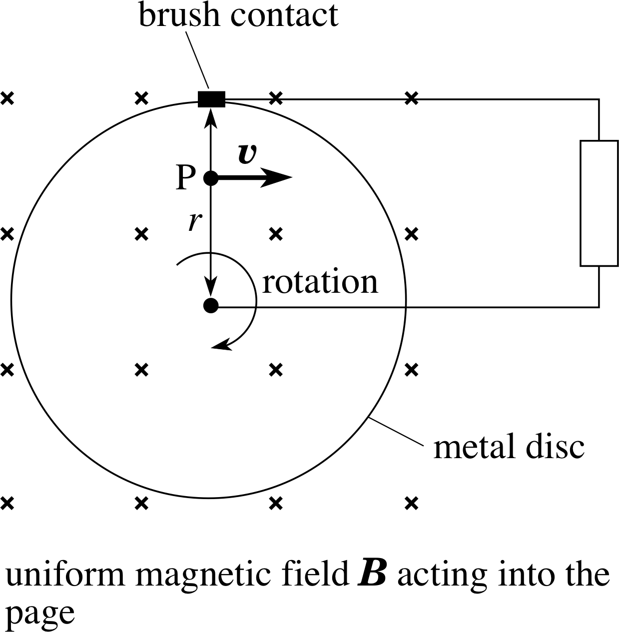
Figure 20 A homopolar generator.
The discussion in the previous subsection can be extended to conductors that rotate in a magnetic field. Figure 20 shows a homopolar generator, i invented by Faraday, which generates a steady d.c. voltage between its centre and rim as the disc rotates.
Imagine the disc consisting of spokes, like a bicycle wheel. Each spoke is moving at 90° to a magnetic field, so we should expect to find an induced voltage between its ends, i.e. between the hub and rim of the disc. To find the magnitude of the voltage, we can write Equation 36,
$V_{\rm ind} = B\dfrac{\Delta A}{\Delta t} = Bl\dfrac{\Delta x}{\Delta t} = \upsilon Bl$ (magnitudes only)(Eqn 36)
in calculus notation as:
$V_{\rm ind} = B\dfrac{dA}{dt}$ (magnitudes only)(37)
Equation 37 is valid for any geometry in which a conductor sweeps across a constant magnetic field – it is not restricted to linear motion. The following worked example shows how it can be applied to the homopolar generator.
Example 2
The disc in Figure 20 has radius 5.0 cm and makes five revolutions per second within a uniform magnetic field of magnitude 0.20 T. Calculate the magnitude of the voltage induced between the hub and the rim and find its polarity.
Solution
In each revolution, a spoke of length r sweeps out an area A = πr2 = π × (0.050 m)2.
It sweeps out this area five times each second, so:
dA/dt = 5 × π × (0.050)2 m2 s−1 = 3.9 × 10⁻² m2 s−1
and so using Equation 37,
V = 0.20 T × 3.9 × 10−2 m2 s−1 = 7.9 × 10⁻³ V = 7.9 mV
The polarity will be such that it produces a clockwise current around the circuit.
You may feel uncomfortable with the above explanation of the voltage which pretends that the disc is composed of spokes. If so, you will be relieved to know that we can arrive at the same conclusion using the Lorentz force law. Equation 33,
Lorentz force law: F = q (E + υ × B)(Eqn 33)
shows that for an electron at P the vector υ × B is directed radially outwards towards the rim, so the force on the electron (q = −e) is radially inwards towards the centre. This is true for any electron in the disc and at any position of the disc. If electrons move towards the centre then the rim develops a positive potential with respect to the centre and the direction of conventional current within the disc is from centre to rim. If the generator is then connected to some external circuit, the flow of positive current from the disc is away from the rim and back to the centre through the circuit, i.e. clockwise around the circuit in Figure 20, which is consistent with the rim being the positive terminal of a generator. If you are worried that within the disc, the conventional current appears to flow from negative to positive then remember that this is exactly what appears to happen inside a battery, when it is connected to some external circuit.
This example shows that, if a disc of area A rotates at frequency f, then the induced voltage has magnitude
Vind = BAf(38)
Question T13
A metal rod of length 2.00 m is spun about one end, around an axis perpendicular to the rod, at a uniform angular speed of 2.00 rad s−1 so that it sweeps out a horizontal circle. The vertical component of the Earth’s magnetic field is Bv = 45.5 μT downwards and the rod spins anticlockwise when viewed from above. Find the magnitude and polarity of the induced voltage in the rod.
Answer T13
Vind = Bv × (horizontal area swept out per second) = BvAf where A is the horizontal area swept out per revolution and f the number of revolutions per second.
A = π × (2.00 m)2 and f = ω/2π = (2.00/2π) Hz
So:Vind = 45.5 × 10⁻⁶ T × π × (2.00 m)2 × (2.00/2π) s−1 = 0.182 mV
From (υ × B), the Lorentz force is towards the centre of the rod and so the centre of the rod will be positive with respect to the tip.
5.3 Eddy currents
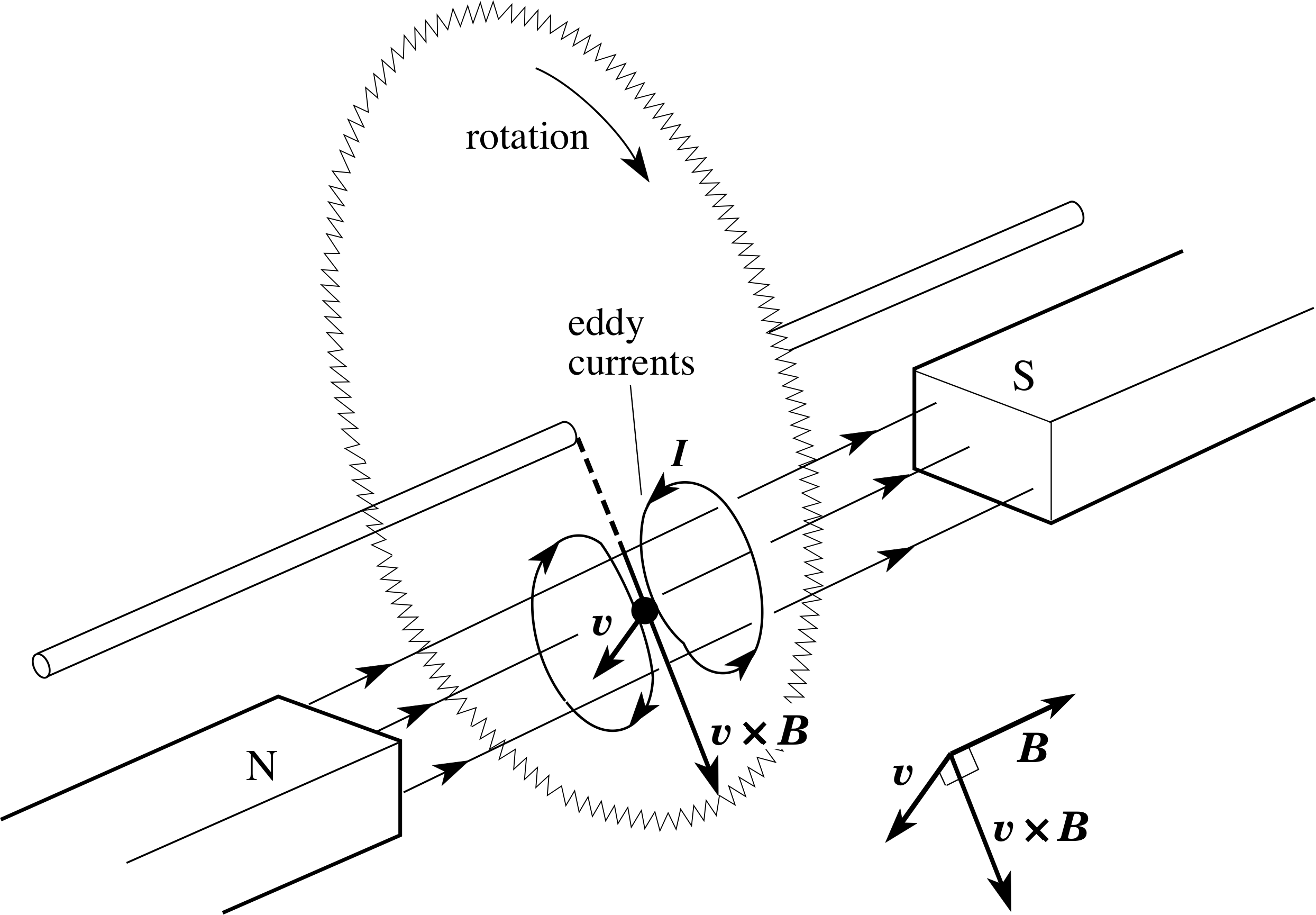
Figure 21 A circular saw rotating between the poles of a magnet.
Figure 21 shows a circular saw rotating between the poles of a magnet. It is similar to the homopolar generator, except that the field extends only over part of the saw and there is no external circuit. As in Figure 20, a voltage is induced that drives conventional current radially outwards. Now, though, the only return path for the current is within the saw itself. An induced current which circulates entirely within the body of a conductor is called an eddy current.
In this particular case, the eddy current can have a useful purpose. From Lenz’s law, the direction of the eddy currents must be such as to provide a force which opposes the motion and so it provides a braking force on the saw. Eddy currents are widely used to provide braking where mechanical contact between moving parts is difficult or undesirable, e.g. for safety reasons or where large frictional forces would cause rapid wear.
Eddy currents may be induced within any conductor in which there is a varying magnetic flux. If a coil is wound on a metal core and the whole is subject to a changing flux, then the changes in flux induce currents within the core itself, as well as in the coil. Sometimes these eddy currents are deliberately suppressed. For example, in the cores of transformers the iron material is composed of many thin insulated sheets. The poor electrical contact between these sheets resists the circulation of eddy currents between the layers, reducing the heating and electrical power loss these would cause. The other extreme is where eddy currents are used to heat a conductor deliberately – most dramatically in an induction furnace, where conducting materials, such as steel, are placed in non–conducting containers and heated to melting temperatures by the eddy currents produced in them when the whole is placed in the high frequency a.c. field of a coil. Such furnaces deliver the heat directly to the conducting materials, not to the container, and since there is no direct contact with the source of heat, there is no contamination.
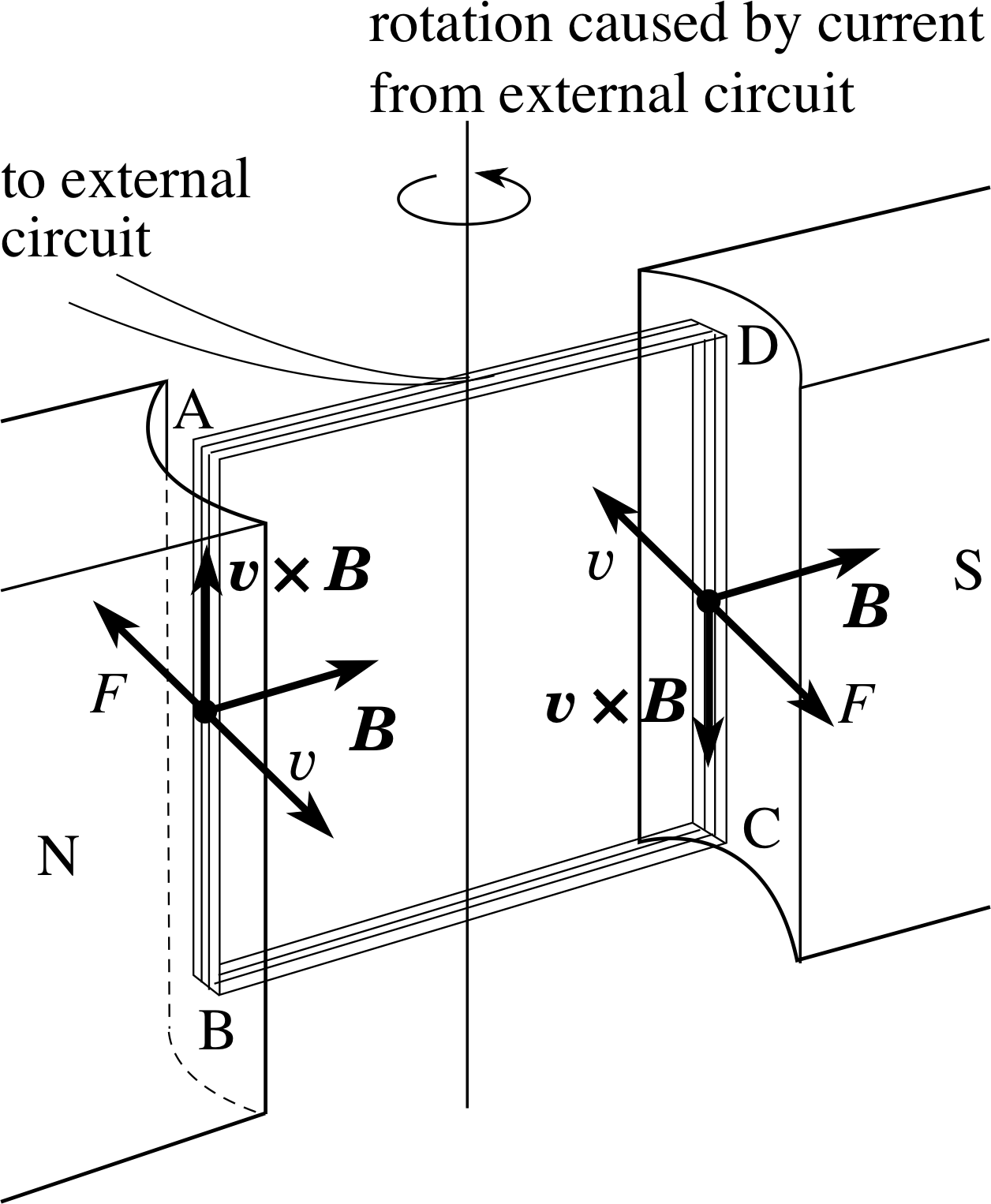
Figure 22 See Question T14.
Question T14
A simple ammeter consists of a vertical rectangular coil, wound on a light metal strip and suspended in a radial magnetic field (a section of this is shown in Figure 22). A current in the coil causes it to rotate anticlockwise when viewed from above.
In what direction is the eddy current induced in the metal strip? What effect does the eddy current have on the motion of the coil? This metal strip was introduced deliberately into the meter design so that eddy currents are induced when the coil moves. What do you think might be a reason for this design feature?
Answer T14
The Lorentz force law gives the direction of the eddy currents as circulating clockwise as viewed in the diagram (i.e. BADC). Lenz’s law shows that the forces due to these eddy currents act ‘into the page’ on side AB and ‘out of the page’ on side CD, i.e. they oppose the coil’s rotation. The forces due to the eddy current are desirable because they slow down (damp) the motion of the coil and prevent repeated overshoots of the final deflection. The coil quickly comes to rest and gives a steady reading rather than swinging back and forth many times before settling. The induction only acts during the motion, so it does not influence the steady state deflection.
6 Closing items
6.1 Module summary
- 1
-
Electromagnetic induction is the process by which an induced voltage is produced either by the motion of a conductor through a magnetic field or by changes in the magnetic field experienced by a circuit.
- 2
-
In a complete circuit of resistance R, an induced voltage gives rise to an induced current
$I_{\rm ind} = \dfrac{V_{\rm ind}}{R}$(Eqn 1)
- 3
-
Lenz’s law states that the polarity of any induced voltage or the direction of any induced current is such as to oppose the change causing it. Similarly, any forces resulting from the induced current are such as to oppose the changes that produced the voltage.
- 4
-
Lenz’s law is a consequence of the principle of conservation of energy.
- 5
-
The magnetic flux ϕ through a loop of area A whose axis makes an angle θ with a uniform magnetic field B is given by
ϕ = BA cos θ(Eqn 3)
- 6
-
Faraday’s law of electromagnetic induction states that the magnitude of the induced voltage in a circuit is equal to the rate of change of the magnetic flux linking the circuit, i.e.
$V_{\rm ind} = \dfrac{d{\it\Phi}}{dt}$(Eqn 7)
where Φ = Nϕ and N is the number of turns of the coil.
- 7
-
The behaviour of alternators, and dynamos is understood in terms of Faraday’s law and the flux linkage changes produced in a coil rotating in a magnetic field.
- 8
-
A sudden finite change in magnetic flux linkage produces a pulse of current in a circuit, in which the total charge flowing past a point in the circuit is proportional to the change in flux linkage. This property is exploited to measure magnetic field strength using a search coil, together with either a ballistic galvanometer or a fluxmeter.
- 9
-
Transformers are devices which use the induced voltage generated in a secondary coil when the current in an adjacent primary coil is changed. To increase the magnetic coupling between the two coils they are usually wound on a common core made from material of high relative permeability.
- 10
-
Transformers are used mainly to change a.c. voltages and in this use their performance is determined by their turns ratio
$\dfrac{V_{\rm s}}{V_{\rm p}} = \dfrac{N_{\rm s}}{N_{\rm p}}$(Eqn 14)
Transformers find many applications, such as d.c. isolation and impedance matching.
- 11
-
The magnetic coupling between two coils is measured by their mutual inductance, which determines the induced voltage in one when the current changes in the other:
$V_{\rm s} = M_{\rm sp}\left\vert\,\dfrac{dI_{\rm p}}{dt}\,\right\rvert$(23a)
and$V_{\rm p} = M_{\rm ps}\left\vert\,\dfrac{dI_{\rm s}}{dt}\,\right\rvert$(23b)
- 12
-
The magnetic coupling within a single coil induces a Lenz’s lawback voltage within the coil itself. This is measured by its self inductance, which determines the magnitude of the induced voltage when the current changes:
$V_{\rm ind} = V_L = L\,\left\lvert\,\dfrac{dI}{dt}\,\right\rvert$(Eqn 17)
This self induction may be exploited to produce a short–lived high voltage from a low voltage source.
- 13
-
The size and polarity of an induced voltage due to motional induction may be found by considering the Lorentz force (electromagnetic force) on the conduction charges:
F = q (E + υ × B)(Eqn 33)
Conventional induced current always flows in the direction of the vector (υ × B).
- 14
-
A homopolar generator uses a conducting disc rotating in a magnetic field to produce a steady d.c. voltage.
- 15
-
Changing the flux within a conductor may induce eddy currents within the conductor itself. Heating due to eddy currents may be useful (e.g. the induction furnace) or a problem (e.g. the energy dissipation in a transformer) and forces due to eddy currents may be exploited to produce braking forces.
6.2 Achievements
Having completed this module, you should be able to:
- A1
-
Define the terms that are emboldened and flagged in the margins of this module.
- A2
-
Recognize the circumstances in which electromagnetic induction occurs and explain, qualitatively, the operation of devices that use it.
- A3
-
Use Lenz’s law to determine the polarity of an induced voltage and the direction of an induced current.
- A4
-
Calculate the magnetic flux linkage in a circuit.
- A5
-
Use Faraday’s law of electromagnetic induction to deduce the magnitude of an induced voltage.
- A6
-
Deduce magnetic field strength from experiments with a search coil.
- A7
-
Apply the relationships between voltage, current and numbers of turns in the primary and secondary coils of a transformer.
- A8
-
Explain the action of an inductance in a circuit
- A9
-
Calculate coefficients of self and mutual inductance for solenoids.
- A10
-
Derive and apply the relationship between the induced voltage in a moving wire, the local magnetic field strength and the wire’s velocity.
- A11
-
Show that Faraday’s law of electromagnetic induction is consistent with the Lorentz force on a conduction charge in a moving wire.
- A12
-
Determine the polarity of the voltage induced and the direction of the current induced in a wire which is moving through a magnetic field.
- A13
-
Explain the principles of an alternator (and how it can be modified to make a d.c. dynamo) and of a homopolar generator.
- A14
-
Explain the origin of eddy currents and appreciate some of their uses and disadvantages.
Study comment You may now wish to take the following Exit test for this module which tests these Achievements. If you prefer to study the module further before taking this test then return to the topModule contents to review some of the topics.
6.3 Exit test
Study comment Having completed this module, you should be able to answer the following questions, each of which tests one or more of the Achievements. i
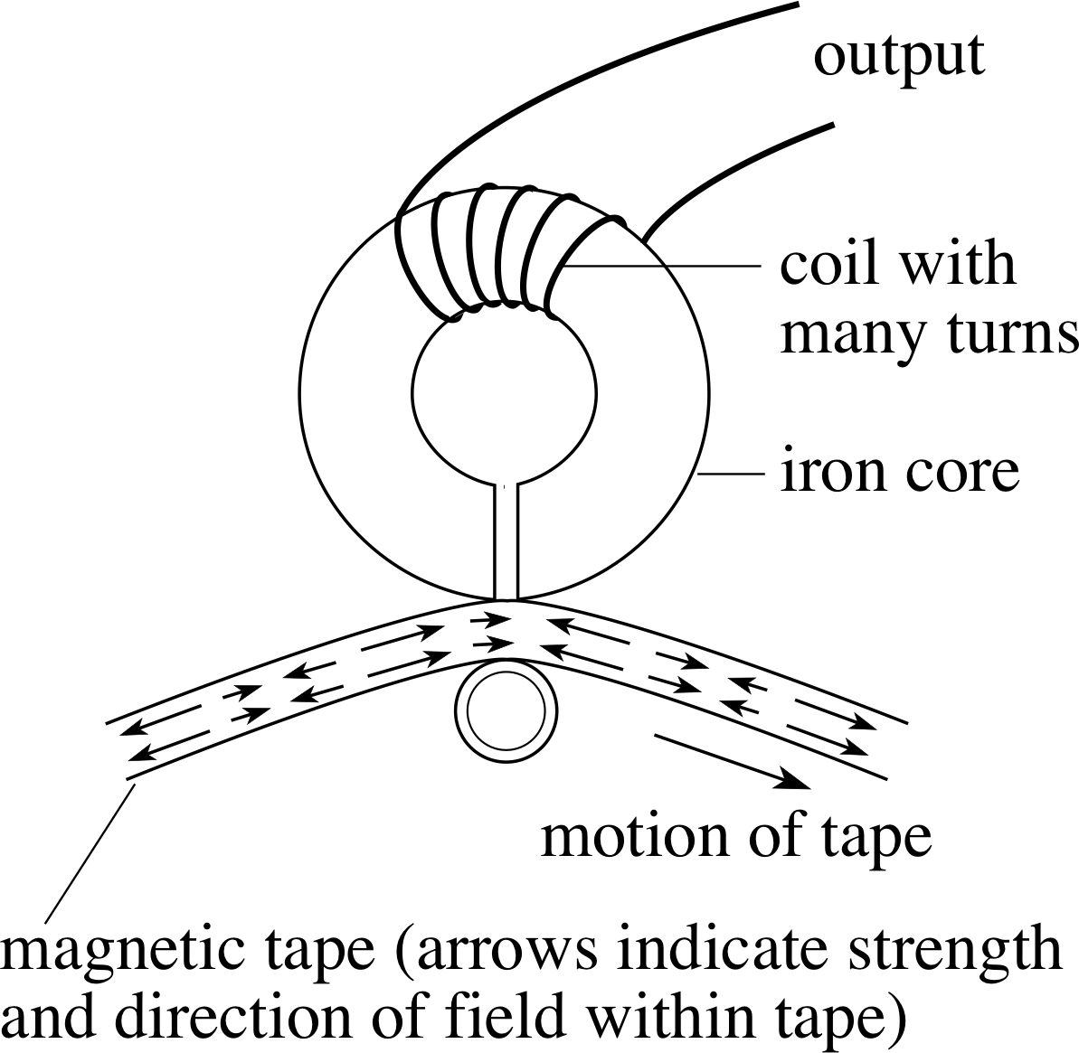
Figure 23 See Question E1.
Question E1 (A2)
Figure 23 is a schematic diagram of the playback head in a tape recorder. Information is stored on the tape in the form of a magnetic field pattern (possibly produced by the output from a microphone). Explain what happens to the output voltage as the tape moves past the head.
Answer E1
The moving tape changes the magnetic field within the iron core and hence changes the magnetic flux linking the coil. The output is a varying voltage induced in the coil by the changing flux.
(Reread Subsection 2.1 if you had difficulty with this question.)
Figure 11 A simple alternator.
Question E2 (A2, A3, A5, A12 and A13)
Figure 11 shows a simple alternator and Figure 13 shows the total flux linkage as the coil turns.
Figure 13 The flux linkage changes as the alternator coil rotates.
If a particular coil makes one full rotation every 40 ms and the voltage output oscillates between ±1 V:
(a) Sketch a graph of the output voltage for two full cycles.
(b) Explain how Lenz’s law and the Lorentz force can each be used to find the direction of the induced current when the coil is moving through the position shown in Figure 11.
(c) On your sketch from (a) show how the output will change if the rotation frequency of the coil is doubled.
Answer E2
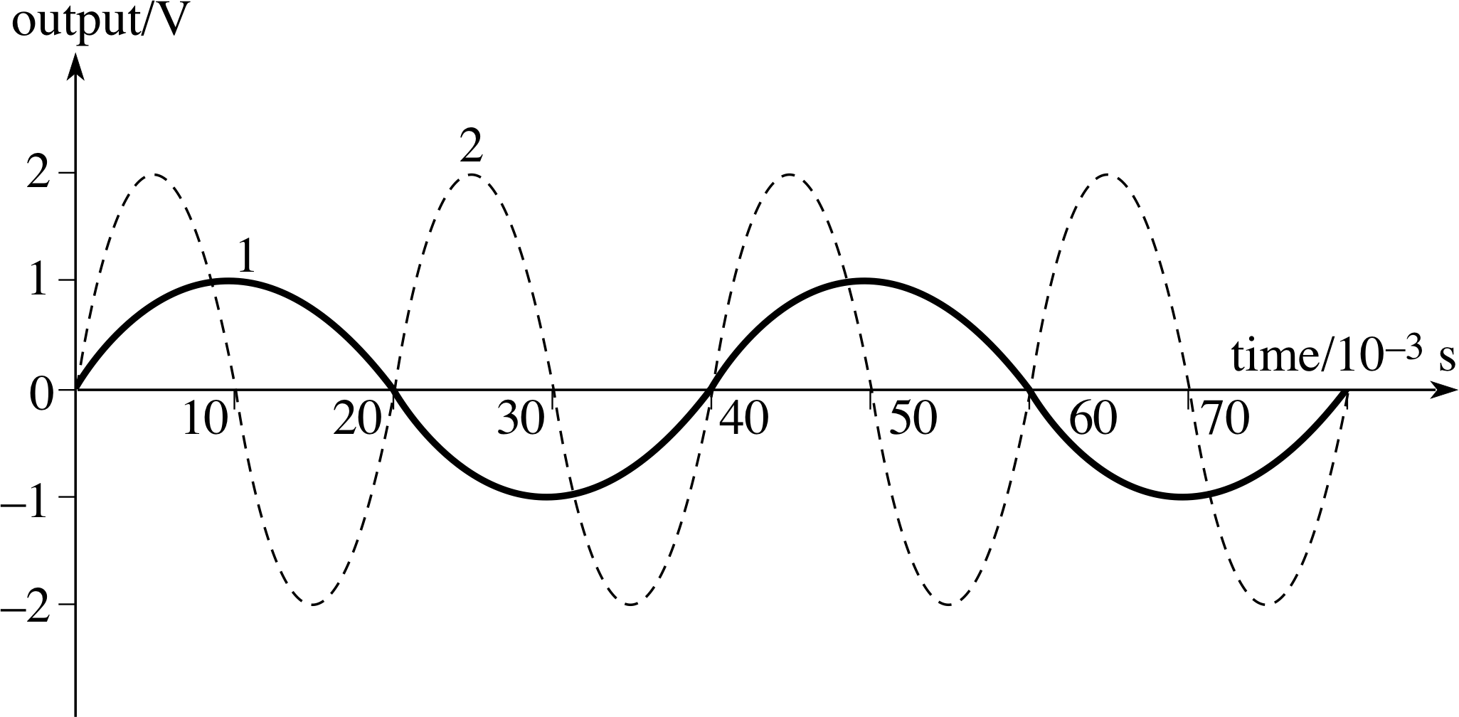
Figure 27 See Question E2.
(a) See curve 1 on Figure 27. The initial voltage is zero since dΦ/dt = 0 at t = 0.
(b) From Lenz’s law: the induced current will ‘try’ to maintain the same amount of flux through the coil. To do this, the right–hand grip rule shows that current needs to circulate around the coil clockwise when viewed from above. From the Lorentz force: at the moment shown in the figure the motion of the lower part of the coil has a downward component of velocity as side Q moves across the field from right to left in the diagram. The vector (υ × B) therefore has a component along the coil towards the observer and so this is the direction of the induced current along Q, i.e. clockwise around the loop, as before.
(c) See curve 2 on Figure 27. The rate of change of flux linkage will be doubled and so the peak induced voltage will double; there are twice as many rotations per second, hence the induced voltage has twice the frequency.
(Reread Subsections 2.2, 3.1, 3.2 and 5.1 if you had difficulty with this question.)
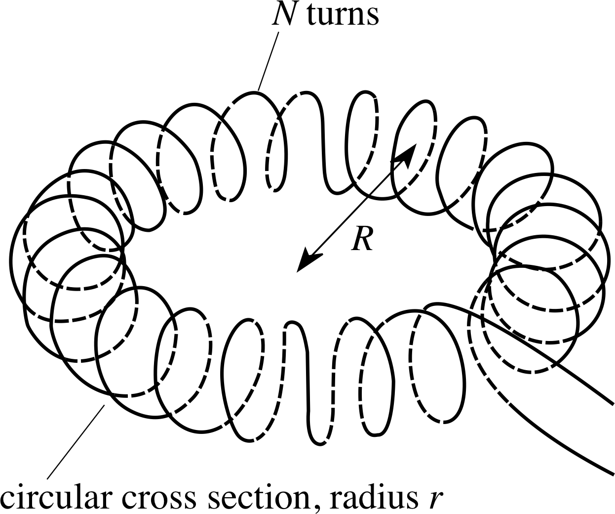
Figure 24 See Question E3.
Question E3 (A4, A5 and A9)
Figure 24 shows a toroidal solenoid. The magnetic field strength at each point on the circular axis of the ring is given by B = μ0NI/(2πR).
(a) If R = 1.0 m, N = 20 000 turns, I = 1.0 A and the circular cross section of the toroid has a radius r = 2.0 cm, calculate the magnetic flux crossing a section of the toroid. (Assume the magnetic field strength B to be uniform across the section.)
(b) If the current in the solenoid grows at the rate of 12 A s−1 calculate the voltage induced in one turn of the solenoid.
(c) Calculate the total induced voltage in the solenoid.
(d) Calculate the total coil inductance L.
Answer E3
(a) From Equation 2,
ϕ = BA(Eqn 2)
the flux within the coil is:
ϕ = BA = [μ0NI/(2πR)] × πr2 = 4π × 10−7 H m−1 × 20 000 × 1.0 A × π (2.0 × 10⁻² m)2/(2π × 1.0 m) = 5.0 × 10⁻⁶ Wb
(b) When I = 1.0 A, the flux linking one turn is 5.0 × 10⁻⁶ Wb, so when the current changes at 12 A s−1, the rate of change of flux linkage is 12 × 5.0 × 10−6 Wb s−1, i.e. (by Equation 7)
Faraday’s law: $V_{\rm ind} = \dfrac{d\Phi}{dt}$(Eqn 7)
each turn has an induced voltage Vind = 6.0 × 10⁻⁵ V.
(c) Total induced voltage = NVind = 1.2 V
(d) Using Equation 17,
$V_{\rm ind} = L\,\left\lvert\,\dfrac{dI}{dt}\,\right\rvert$(Eqn 17)
when | dI/dt | = 12 A s−1, Vind = 1.2 V, and so L = 0.10 H.
(Reread Subsections 3.1 and 4.2 if you had difficulty with this question.)
Question E4 (A4 and A6)
In an early experiment to measure the strength of the Earth’s magnetic field, a large flat vertical coil of 400 turns and radius 30 cm, with its axis pointing to magnetic north, was turned through 180° about a vertical diameter. The coil was connected to a ballistic galvanometer which measured a charge flow of 49.2 μC when the coil was turned round. The total resistance of the circuit was 200 Ω.
(a) Calculate the magnitude Bh of the horizontal component of the Earth’s magnetic field strength.
(b) How should the coil be positioned and turned to measure the vertical component of the Earth’s magnetic field strength?
Answer E4
(a) The flux through the coil changes from maximum to zero then to a negative maximum, so Equation 12,
$\Delta q = \langle V_{\rm ind}\rangle\Delta t = \dfrac{\Delta{\it\Phi}}{R} = \dfrac{BAN}{R}\cos(\theta)$(Eqn 12)
gives the charge ∆q = 2NBhA/R so
Bh = 200 Ω × 49.2 × 10−6 C/(2 × 400 × π × (0.30 m)2) = 4.35 × 10⁻⁵ T
(b) The coil should be laid flat and turned about a horizontal diameter.
(Reread Subsections 3.1 and 3.3 if you had difficulty with this question.)
Question E5 (A7 and A9)
A ring–shaped transformer consists of a primary coil of 12 turns cm−1 and cross–sectional area 6.0 cm2, wound completely around the ring (as in Figure 24) with a superimposed secondary coil of 3000 turns in total, also wound completely around the ring. The ring has radius R = 15 cm and the material of the core has relative permeability μr = 500. Assume this transformer to be ‘ideal’.
(a) If there is an alternating voltage of 240 V across the primary coil, what is the output voltage from the secondary?
(b) How could this transformer be used to step down an a.c. voltage of 240 V, and what would then be the output voltage?
(c) Calculate the coefficient of mutual induction of this transformer.
Answer E5
(a) The ring has circumference 2πR = 30π cm, so the number of turns in the primary coil is Np = 12 × 30π = 1131 (nearest whole number).
From Equation 14,
For an ideal transformer: $\dfrac{V_{\rm s}}{V_{\rm p}} = \dfrac{d{\it\Phi}_{\rm s}/dt}{d{\it\Phi}_{\rm p}/dt} = \dfrac{N_{\rm s}(d\phi_{\rm s}/dt)}{N_{\rm p}(d\phi_{\rm p}/dt)} = \dfrac{N_{\rm s}}{N_{\rm p}}$(Eqn 14)
secondary voltage Vs = Vp × (Ns/Np) = 240 V × 3000/1131 = 6.4 × 10² V
(b) By using the 3000 turn coil as the primary, and the other as the secondary, the voltage would be stepped down by a factor of 1131/3000 = 0.377. The output voltage would then be 0.377 × 240 V = 90.5 V.
(c) Since ls = lp = l, Equations 31 and 32,
P–S mutual inductance$M_{\rm ps} = \dfrac{\mu_{\rm r}\mu_0AN_{\rm p}N_{\rm s}}{l_{\rm s}}$(Eqn 31)
S–P mutual inductance$M_{\rm sp} = \dfrac{\mu_{\rm r}\mu_0AN_{\rm p}N_{\rm s}}{l_{\rm p}}$(Eqn 32)
give:
Mps = Msp = M = (μrμANpNs/l)
and using Np/l = 12 cm−1 = 1.2 × 10³ m−1
M = 500 × 4π × 10−7 H m−1 × 6.0 × 10−4 m2 × 1.2 × 103 m−1 × 3000 = 1.4 H
(Reread Subsections 4.1, 4.2 and 4.3 if you had difficulty with this question.)
Question E6 (A8 and A14)
A coil of several hundred turns is wound on to a solid iron core. When the coil is connected in series with a lamp and a 12 V battery, the lamp glows brightly. When the same lamp and coil are connected to a 12 V a.c. supply, (a) the lamp barely glows at all and (b) the coil becomes very hot. Suggest an explanation for each of the observations (a) and (b).
Answer E6
(a) When an a.c. supply is used, the changing current changes the flux within the coil, which gives rise to a self induced voltage (a back voltage). The direction of this voltage is such as to oppose the change causing it, so the net voltage across the lamp is much less than 12 V and the lamp cannot light with its normal brightness.
(b) The changing flux induces eddy currents that circulate within the solid iron core, causing heating.
(Reread Subsections 4.2 and 5.3 if you had difficulty with this question.)
Study comment This is the final Exit test question. When you have completed the Exit test go back and try the Subsection 1.2Fast track questions if you have not already done so.
If you have completed both the Fast track questions and the Exit test, then you have finished the module and may leave it here.
Study comment Having seen the Fast track questions you may feel that it would be wiser to follow the normal route through the module and to proceed directly to the following Ready to study? Subsection.
Alternatively, you may still be sufficiently comfortable with the material covered by the module to proceed directly to the Section 6Closing items.