PHYS 7.1: The atomic basis of matter |
PPLATO @ | |||||
PPLATO / FLAP (Flexible Learning Approach To Physics) |
||||||
|
1 Opening items
1.1 Module introduction
In these days of nuclear power and pictures claiming to show individual atoms, it is very easy to take the existence of atoms for granted. Yet, although the philosophical concept of atoms was discussed by Leucippus and Democritus over two thousand years ago, atoms as a scientific fact did not become widely accepted until this century, and our current understanding wasn’t essentially completed until Chadwick discovered the neutron in 1932. It may be difficult to conceive of an understanding of matter that doesn’t include atoms, because we now frame our fundamental explanations of the properties of bulk matter in terms of the structure of atoms and molecules and the forces that act between them.
One can imagine two motivations for the development of the idea of atoms. The first was the desire on the part of both chemists and physicists to probe the fundamental nature of matter and to identify its most elementary constituents. This same desire currently motivates particle physicists to understand how quarks make up the protons and neutrons which (together with electrons) form atoms. A second motivation was the desire to explain and, if possible, quantitatively predict the properties of gases, liquids and solids in terms of the more elementary properties of their constituent atoms. This modelling in terms of atomic properties allows for a deeper insight into the macroscopic i properties of matter.
In Section 2, we consider the development of ideas about the nature of atoms, from the early philosophical speculations to more recent, but still vague, scientific speculations. In the course of this, we discuss Avogadro’s hypothesis about the nature of gases and the scale of atomic sizes indicated by Avogadro’s constant.
In Section 3 we outline various phenomena and experiments which provide us with proof of the existence of atoms and reveal their size and properties; these include Brownian motion, X–ray diffraction, and the use of modern instruments such as the scanning tunnelling microscope and the atomic force microscope, which actually allow us to form images of individual atoms on surfaces.
In Section 4 we discuss more precise ideas about atoms and molecules and their interactions (the forces that act between them). We use models formulated in terms of classical physics to discuss the bonding that holds atoms together, and give a brief introduction to the more modern formulations of quantum physics. Finally, we briefly consider the nature of gases, liquids and solids, the three common phases of matter, and explain how they can be pictured in terms of atoms and molecules and their interactions.
Study comment Having read the introduction you may feel that you are already familiar with the material covered by this module and that you do not need to study it. If so, try the following Fast track questions. If not, proceed directly to the Subsection 1.3Ready to study? Subsection.
1.2 Fast track questions
Study comment Can you answer the following Fast track questions? If you answer the questions successfully you need only glance through the module before looking at the Subsection 5.1Module summary and the Subsection 5.2Achievements. If you are sure that you can meet each of these achievements, try the Subsection 5.3Exit test. If you have difficulty with only one or two of the questions you should follow the guidance given in the answers and read the relevant parts of the module. However, if you have difficulty with more than two of the Exit questions you are strongly advised to study the whole module.
Question F1
State Avogadro’s hypothesis. What is the significance of Avogadro’s constant?
Answer F1
Avogadro’s hypothesis: equal volumes of gases at a specified temperature and pressure contain the same number of molecules. Avogadro’s constant specifies the number of atoms or molecules that are in one mole of any substance.
Question F2
Bragg’s law can be stated as nλ = 2d sin θ. Briefly explain the meaning of the terms in this equation.
Answer F2
θ is the angle between the atomic planes and the incident radiation; d is the perpendicular spacing between the atomic planes; λ is the wavelength of the radiation and n is the order of the reflection from the planes with a given spacing.
Question F3
Describe qualitatively the differences between the gas, liquid and solid phases of a substance in terms of intermolecular distances and energies.
Answer F3
In a gas, the molecules are comparatively far apart, and hence the forces acting between molecules are negligible. In liquids, the molecules are much closer together, essentially touching, so that the intermolecular forces are very important, but the molecular energies are large enough that they don’t settle down into a stable ordered arrangement. In solids, the distances are similar to those in liquids, with the forces being very important, but the molecular energies are small enough that the molecules can settle into oscillating about fixed equilibrium positions. In a crystalline solid the equilibrium positions form a regular array.
1.3 Ready to study?
Study comment In order to study this module you will need to be familiar with the following terms from mechanics and electrostatics: electric dipole, electric field, equilibrium, force, kinetic_energykinetic and potential energy. If you are uncertain about any of these terms, review them in the Glossary, which will indicate where in FLAP these ideas are more fully discussed. The following Ready to study questions will allow you to establish whether you need to review any of these topics before starting this module.
Question R1
Describe the qualitative nature of the force that acts between an electron and a proton at a fixed separation. How does this compare with the force between two electrons at the same separation?
Answer R1
The electron and proton experience an electrostatic force. Because the charges have opposite signs, the force will be attractive, and act along the line between the two particles. The force between two electrons will have the same magnitude at the same separation, but will be repulsive, tending to force the two electrons apart.
Consult the relevant terms in the Glossary for further information.
Question R2
A particle experiences a force which is attractive at large distances from a source and repulsive at small distances. Under these circumstances, there will be a position of stable equilibrium for this particle. Explain what this expression means, and describe qualitatively at what distance from the source this position will occur.
Answer R2
Stable equilibrium means that there is no net force acting on the particle, and if it moves away from that position, the force that acts will tend to push it back to the point of stable equilibrium. In the case of a force which is attractive at large distances and repulsive at smaller distances, the force changes sign as the distance changes. This means that it must become zero at some position, and this will be the equilibrium point.
Consult stable equilibrium in the Glossary for further information.
2 The concept of an atom
2.1 Models of matter
The earliest recorded concept of an atom, as the smallest indivisible component of matter, is probably due to the Greek philosopher Leucippus i and his student Democritus i in the 5th century BC. They proposed that all matter is made up of innumerable atoms, all with identical composition, existing and moving in the void. The various forms of substance that we see around us are then simply the result of endless combinations of these fundamental entities (in the same way that a pile of bricks can be used to build an endless variety of houses or other buildings). This point of view was in opposition to the concept that one could continually split matter into smaller parts, never reaching an end and never coming upon a new level of matter which was qualitatively different. These different views of the nature of the physical world represent an enduring intellectual conflict in the human attempt to understand the physical universe, reflected in current physics by the particle/wave dichotomy.
The concept of an atom actively entered modern science at the start of the 19th century through the work of chemists and physicists. Chemists used the concept to help organize their experimental results concerning chemical reactions and the relationship between elements and compounds. In the 19th century, an element was regarded as a chemical substance that could not be broken down by heating or passing electrical currents through a sample. Compounds were less well defined but were widely regarded as substances in which elements were more intimately combined than in a simple mixture. The law of definite proportions, proposed by J. L. Proust in 1800, i attempted to clarify the nature of compounds by supposing that any chemical compound contains a fixed and constant proportion (by mass) of its constituent elements.
✦ A chemist finds that 2 g of hydrogen will combine completely with 16 grams of oxygen to form 18 g of water. According to the law of definite proportions, what will be the amounts of hydrogen and oxygen required to form 9 g of water?
✧ The chemist’s finding shows that the proportion of hydrogen in water is 2/18 = 1/9 (by mass), and that of oxygen is 8/9. Therefore (1/9) × 9 g = 1 g of hydrogen is required, and (8/9) × 9 g = 8 g of oxygen.
Question T1
This same chemist finds that sometimes 3 g of carbon will react fully with 4 g of oxygen, while at other times his measurements indicate that 3 g of carbon react fully with 8 g of oxygen. What can be concluded from this data, according to the law of definite proportions?
Answer T1
Since the proportions of the carbon and oxygen are different for the two cases (3/7 and 4/7 for one case, and 3/11 and 8/11 for the other), there must be (at least) two different compounds that can form from carbon and oxygen.
In 1808, partly motivated by Proust’s law, John Dalton i expressed the idea that all matter was composed of atoms, with each element having a distinctive kind of atom with its own characteristic mass. According to this view compounds resulted when atoms combined to form molecules, which suggested that molecules were composed of whole numbers of atoms of the appropriate elements.
Question T2
The chemist from Question T1 believes that when 3 g of carbon reacts with 4 g of oxygen, the resulting compound has one atom of each element per molecule. If that is true, what can we say about the number in a molecule formed by 3 g of carbon and 8 g of oxygen?
Answer T2
If the first compound has one oxygen per carbon atom, then the second must have two oxygen atoms for each carbon. These correspond then to CO (carbon monoxide) and CO2 (carbon dioxide).
With the ideas of Dalton and his supporters, we have the characteristics of a modern scientific explanation: the proposed atomic model of matter explained existing observations, provided a general framework for a range of ideas, and suggested further measurements that might support or refute the theory.
William Prout i further hypothesized in 1815 that all elements were composed of combinations of a single fundamental particle, the atom of hydrogen. Although this speculation was incorrect, it is in some respects close to the modern understanding of atomic nuclei as being made up of protons (which are hydrogen nuclei) and neutrons (which have virtually the same mass). Of course, Prout was unaware of the existence of these particles, just as he was unaware of the existence of electrons, which balance the nuclear charge and are responsible for most of the distinctive chemical and physical properties of each element.
At around the same time, Amedeo Avogadro i was developing an hypothesis about the number of atoms or molecules in a quantity of gas, that would eventually simplify the determination of the masses of many molecules. We will discuss this in detail in the next subsection since it has survived as a cornerstone of modern science, but it should be noted, however, that many chemists of the time still considered the idea of atoms to be nothing more than a bookkeeping tool for analysing chemical reactions.
Physicists invoked the idea of atoms to explain the observed properties of matter, especially with regards to the behaviour of gases as their temperature and pressure changed. In the 18th and 19th centuries, understanding the thermal behaviour of gases was not only at the forefront of pure research, but was crucial to the development of technology in the revolution of steam power. The science of thermodynamics developed laws of the macroscopic behaviour of matter that allowed technology to advance, but failed to explain these laws in terms of more fundamental entities. The kinetic theory of matter represented an attempt to understand the thermal properties of gases in terms of the existence and motion of microscopic atoms. In the 18th century, Daniel Bernoulli i introduced the hypothesis that the mechanical collisions of particles with the walls of containers were responsible for the existence of gas pressure. In the early 19th century, Rudolph Clausius i developed the qualitative idea that the difference between solids, liquids and gases can be understood on the basis of differences in their molecular motions. He also began to perform numerical calculations based upon the average molecular motion in a gas.
In the latter half of the 19th century, James Clerk Maxwell i developed the first truly systematic and detailed kinetic theory of gases, which allowed for the random motions of individual molecules but nevertheless predicted the distribution of molecular speeds and related the average speed of a molecule to the temperature of the gas. Ludwig Boltzmann i extended these ideas to other forms of matter, including liquids and solids, and established a general statistical connection between the distribution of molecular kinetic energies and temperature. The mathematical statement of this relationship, the Maxwell–Boltzmann distribution function, is now seen as a key to the classical understanding of the properties of matter.
Boltzmann was a fervent proponent of the statistical theory of matter, which used atoms as a basic ingredient. He was especially concerned about clarifying the connection between Newton’s laws of motion, which were deterministic and predictive (at least as far as was known at the time) and the statistical mechanics of matter, which exhibits probabilistic behaviour. Furthermore, Newton’s laws were reversible in time, while the behaviour of matter often seems irreversible (as in the case of diffusion). Boltzmann played a crucial role in clarifying the relationship between the macroscopic and microscopic views of these issues. Bitter scientific disputes arose about the origin of these irreversible aspects, and were closely intertwined with disputes about the reality of atoms.
2.2 Avogadro’s hypothesis: the mole, relative atomic mass and Avogadro’s constant
What is the mass of an atom or a molecule? Although this question could not be answered until the 20th century, Avogadro, in 1811, had already enunciated a principle which allows the relative masses of the atoms or molecules of different substances to be compared. Avogadro assumed that atoms (or molecules – there wasn’t a clear distinction in his time) exist, and that they are unchanging. Furthermore, he stated that:
Equal volumes of gases at a specified temperature and pressure comprise the same number of elementary entities, such as atoms or molecules.
Now known as Avogadro’s hypothesis, this principle enabled the relative masses of different molecules to be measured simply by weighing large quantities of gas under standard conditions. The standard conditions traditionally used were a pressure of 1 atmosphere, a temperature of 0°C and a volume of 0.022 414 m3, and the amount of gas contained under such circumstances was called a mole. If, for example, 1 mole of oxygen had a mass of 32 g and 1 mole of nitrogen had a mass of 28 g, this would indicate that an oxygen molecule is more massive than an nitrogen molecule by a factor 32/28 = 8/7.
Modern definitions, made since Avogadro’s time, allow his ideas to be used with more precision. First, a particular type of atom is chosen as a reference: this is carbon-12, i the stable atom of carbon with atomic mass 12 (with six protons and six neutrons in its nucleus). A sample of carbon-12 with a mass of 12 g is defined to be a mole of carbon-12 and, inspired by Avogadro’s hypothesis:
A mole of any other substance is a quantity of that substance that contains the same number of elementary entities (atoms or molecules) as are present in the 0.012 kg of carbon-12.
This number is known as Avogadro’s number and has a value of 6.022 045 × 1023. A related physical constant, measured in units of mol−1 is Avogadro’s constant, the number of elementary entities per mole.
Avogadro’s constant NA = 6.022 045 × 1023 mol−1
You may wonder why 6.022 045 × 1023 mol−1 was chosen for NA, rather than something straightforward – like 1.00 × 10²³ mol−1? Believe it or not it was chosen to make things simpler! With this value of NA the mass of one mole of any substance, expressed in grams, is numerically equal to its relative atomic mass or relative molecular mass. This is because one mole of any substance contains the same number of atoms (or molecules) as one mole of carbon-12, so the mass of one mole of any substance is given by:
$\dfrac{\text{mass of one mole of substance}}{\text{mass of one mole of carbon-12}} = \dfrac{\text{average mass of one atom (or molecule) of substance}}{\text{mass of a carbon-12 atom}}$
Since the mass of one mole of carbon-12 is 0.012 kg = 12 g, it follows that the mass of one mole of any substance, measured in grams, is:
$\text{mass of one mole of substance g} = \dfrac{\text{average mass of one atom (or molecule) of substance}}{\frac{1}{12}\times \text{mass of a carbon-12 atom}}$
However, the quantity on the right–hand side is, by definition, the relative atomic (or molecular) mass of a substance. Hence, as claimed:
The mass of one mole of any substance, measured in grams, is numerically equal to the relative atomic (or molecular) mass of that substance.
Question T3
(a) What is the mass of an individual 12C atom?
(b) If the relative atomic mass of a lead atom is 207.2, what is the mass of an individual lead atom?
Answer T3
(a) One mole of atoms contains Avogadro’s number of atoms, so 6.022 × 10²³ atoms have a mass of 12 g. The mass per carbon atom is then:
0.012 kg/6.022 × 1023 = 1.99 × 1026 kg
(b) Similarly, the mass per lead atom is:
0.207 kg/6.022 × 1023 = 3.44 × 1025 kg
3 Evidence for the atomic basis of matter
There are various experimental techniques which provide direct information about the existence and size of atoms. We might mention in the first place the observation that a film of oily substances on the surface of water spreads to cover a finite area and then stops spreading. One conclusion from this is that there is in fact a smallest particle of the substance, otherwise you might expect the film to spread indefinitely. Given the initial volume of the liquid, and the area that the film eventually covers, one can calculate the resulting thickness of the film. This thickness will represent an upper limit to the size of individual molecules in the material.
Question T4
Stearic acid spreads in the way described above. If a drop of stearic acid with a volume of 5 × 10⁻¹² m3 spreads in a film to cover an area of 30 cm2, what is the upper limit to the size of the molecule of stearic acid?
Answer T4
If the stearic acid has a volume of 5 × 10⁻¹² m3 and covers an area of 30 cm2 = 3.0 × 10⁻³ m2, the thickness of the film must be:
5 × 10⁻¹² m3/3.0 × 10−3 m2 = 1.7 × 10⁻⁹ m = 1.7 nm
If the film is a monolayer (i.e. it is one molecule thick), this will be the actual size of the molecule. If there is more than one layer, this number will represent some multiple of the actual molecular size.
3.1 Brownian motion and other statistical phenomena
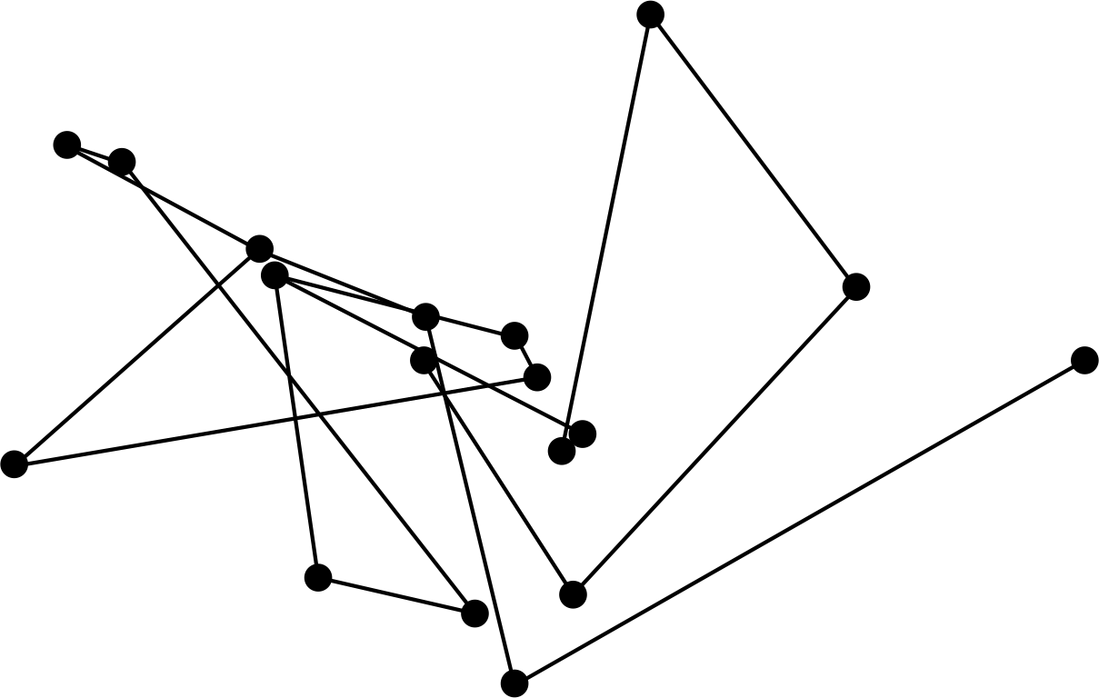
Figure 1 The random path followed by a small grain suspended in water is an example of Brownian motion.
Robert Brown i first observed the apparently random motion (indicated schematically in Figure 1) of pollen grains in water through microscopic observations in 1827. At first, it was believed that the pollen grains were living creatures, but it was soon discovered that the smaller grains moved faster, which seemed to argue against that interpretation. In fact, the random motion (now known as Brownian motion) is generally only observable for particles smaller in diameter than about 10−6 m.
In addition, the study of smoke particles suspended in air showed the same behaviour. Further experimental studies ruled out causes such as temperature gradients, capillary action, irradiation of the liquid, and convection currents as the source of this frenetic activity. In the 1860s, it was suggested by a number of physicists that these random motions were the result of collisions with the molecules of the fluid, which sparked a heated debate about the effects of these microscopic collisions.
In 1905, as well as creating the special theory of relativity and analysing the photoelectric effect, Albert Einstein i studied the statistical effects of molecular impacts on the motion of microscopic particles suspended in a fluid, and arrived at a prediction of behaviour that was similar to that observed in Brownian motion. At that time, Einstein lacked the information to unambiguously identify Brownian motion as the result of the behaviour he had analysed, but in 1908 and the following years Jean Perrin i used this and others of Einstein’s theoretical developments to characterize Brownian motion, and indeed arrive at a value for Avogadro’s constant.
Similar reasoning and calculations arose in a number of areas of physics, all involving phenomena representing fluctuations of some physical quantity. These included measurements of voltage fluctuations in resistors (arising from thermal agitation of electrons), critical opalescence in fluid phase transitions (which are fluctuations of density and hence light scattering power) and Rayleigh scattering in the atmosphere (responsible for the blue colour of the sky). All of these provided independent ways of estimating Avogadro’s constant, and all gave results that (after careful measurement) were in the range of 6–9 × 10²³ mol−1. It was this wide–ranging agreement that finally led to the almost universal acceptance of the actual existence of atoms. (Although Ernst Mach i ultimately died unconverted in 1916, perhaps providing experimental evidence for Bohr’s contention that new physical theories only become fully accepted when the previous generation of scientists has died.)
3.2 X–ray scattering and Bragg’s law
Interference phenomena are familiar from the behaviour of light, and are a general characteristic of all waves. Max von Laue i first proposed an experiment to demonstrate the wave nature of X–rays in 1912. It was founded on the dual ideas that X–rays were a type of wave, and that crystalline solids were formed from regular arrangements of atoms that would serve as a form of diffraction grating. X–ray diffraction was observed by W. Friedrich (1883–1968) and P. Knipping (1883–1935), and thus simultaneously verified both hypotheses. The precise nature of the scattering was then analysed in a simple model by W. L. Bragg i to give a quantitative relationship.
In its simplest form, this model for the scattering assumes that planes of atoms serve to reflect some fraction of an incident X–ray wave. Since X–rays are quite penetrating, many planes of atoms will contribute to observed reflections, so that there will be interference i between reflections from different planes.
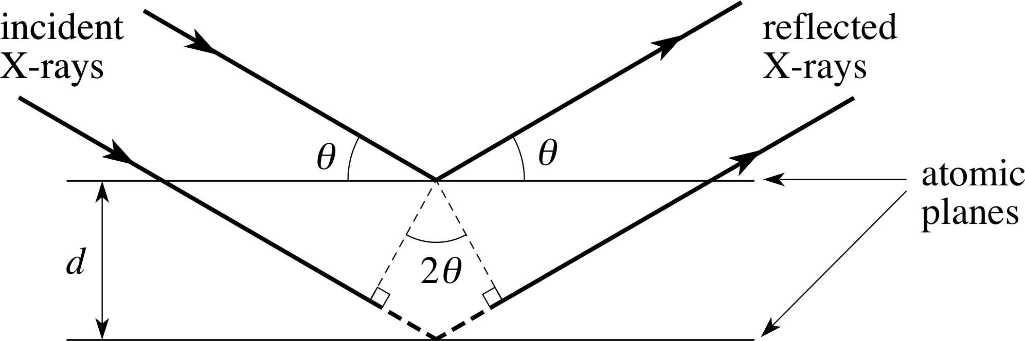
Figure 2 X–rays scattering from planes of atoms exhibit interference effects leading to specific angles where reflections are observed.
This interference will be constructive only if the path difference for reflections from two planes is a whole multiple of the wavelength of the X–ray. This is illustrated in Figure 2.
The diffraction is characterized in terms of two parameters indicated in Figure 2: the angle between the normal to the incident wavefront and the parallel planes of atoms, denoted by θ, i and the perpendicular distance between the atomic planes, denoted by d. The section of path for the reflection from the second plane between the two heavy dashed lines represents the extra distance travelled by the wave during reflection from the second plane. This extra distance is made up of two equal contributions, each being the opposite side to an angle θ in a right triangle which has the perpendicular distance d between the planes of atoms as its hypotenuse.
Trigonometry leads to the result that this dashed side has the length dsin θ, so that the total extra distance travelled is 2d sin θ. If the individual waves are going to add up to produce an amplitude maximum, the extra distance travelled by the second wave must be an integral multiple (n) of the wavelength λ.
This condition ensures that the two reflected waves in Figure 2 emerge a whole number of wavelengths (n) out of step, and so produce constructive interference and a strong signal at the detector. What is more, waves reflected from deeper layers will also be a whole number of wavelengths (2n, 3n, 4n, etc.) out of step and will also interfere constructively. Thus, we have the condition for a maximum in the interference pattern that the wavelength of the X–rays be given by:
Bragg’s law nλ = 2d sin θ(1)
where n is a whole number and d is the spacing between neighbouring atomic planes.
Bragg’s law allows us to calculate the spacing between neighbouring planes of atoms provided we know the wavelength of the X–rays, and the angular positions of the diffraction peaks. The phenomenon of X–ray diffraction serves as experimental evidence for the existence of atoms, and also allows for the quantitative determination of distances between atoms. On the assumption that the atoms in a solid are packed tightly together, like bricks in a house, it also gives an estimate of atomic sizes. Note that one consequence of Bragg’s law is that, if the wavelength is much larger than the spacing, the equation cannot be satisfied, because sin θ cannot be larger than one. On the other hand, if the wavelength is much smaller than the spacing d, then sin θ and hence θ must be very small, meaning that there is in practice no observable pattern. Thus an observable reflected diffraction pattern only occurs for wavelengths that are on the same scale as the atomic spacing in the material.
Question T5
The spacing between a certain set of atomic planes in copper is 0.208 nm. What is the largest wavelength of radiation which can produce a reflection from this set of planes according to Bragg’s law?
Answer T5
The wavelength in Bragg’s law can be expressed as (2d sin θ)/n. The largest value this expression can have is when n = 1 and sin θ = 1. Then λ = 2d = 2 × 0.208 nm = 0.416 nm. For any larger wavelength, there is no reflection from these planes.
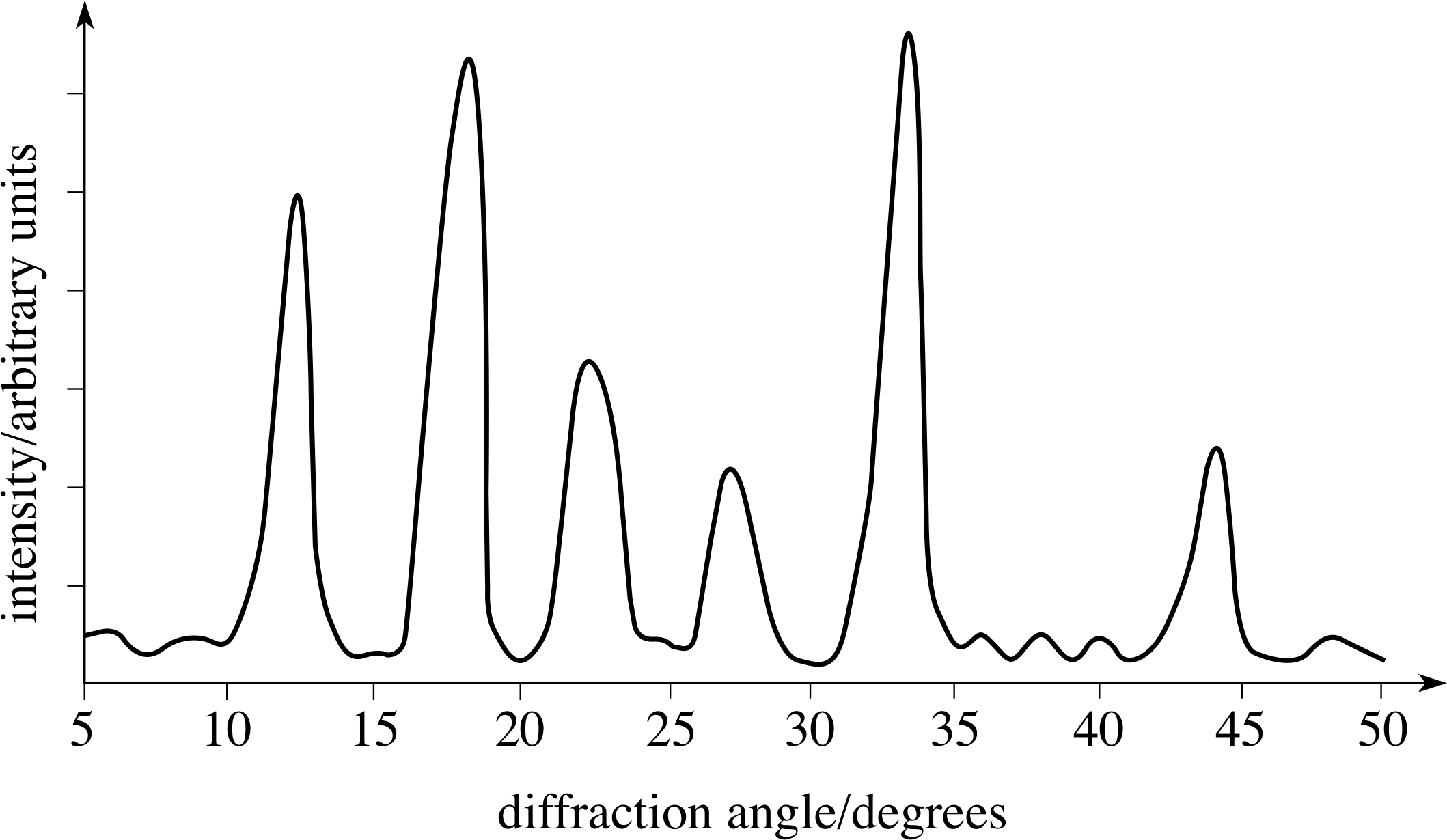
Figure 3 A typical X–ray diffraction pattern.
The X–ray diffraction is observed either using photographic film (which measures an entire pattern simultaneously) or electronic detectors (which usually count at a sequence of angles). An example of a pattern from a counter experiment is shown in Figure 3.
This sort of pattern can be analysed to provide information about various spacings within the substance and this allows the reconstruction of the structure of the atoms or molecules in the material. It has the disadvantage, however, that there are no unique solutions to the problem of identifying the original structure that produces a given diffraction pattern. The analysis can only show that the model is consistent with the experimental result.
3.3 Modern microscopes
It is a fundamental limitation of measurements that use radiation that the smallest scale observable is determined by the wavelength of the radiation used, as exemplified by our discussion of Bragg interference above. Thus, optical microscopes are limited by the wavelength of visible light to examining structures that are no smaller than approximately 10−6 m, and so can provide no evidence for the existence of atoms or molecules. In visible light matter appears to be continuous. However, quantum physics tells us that particles also have a wave nature, and thus can serve as a tool for studying structures. According to the ideas of quantum physics, we can calculate the wavelength λ associated with a particle of momentum of magnitude p using the following formula:
$\lambda = \dfrac hp$
where h is known as Planck’s constant, and has an approximate value of 6.63 × 10⁻³⁴ J s. According to Newtonian mechanics the momentum magnitude p is given by the product mυ, where m is the particle’s mass and υ is its speed, so as m or υ increases, the wavelength decreases.
Electron diffraction makes use of the wave nature of electrons to probe matter with much smaller wavelengths than visible light but the information is indirect, as with X–ray diffraction. Neutron diffraction is a technique that is very similar to X–ray diffraction, but provides elementary information about structures thanks to the differences in the interactions between neutrons and matter on the one hand and X–rays and matter on the other. A drawback to all of these techniques is that the result is a diffraction pattern, which must be mathematically manipulated to provide any information about the spatial distribution of atoms.
Question T6
An electron in an electron diffraction instrument moves with a speed of 1.00 × 10⁷ m s−1. The mass of an electron is 9.11 × 10⁻³¹ kg. What is the quantum mechanical wavelength of such an electron?
Answer T6
The wavelength is given by:
h/mυ = 6.63 × 10⁻³⁴ J s/(9.11 × 10−31 kg × 1.00 × 107 m s−1) = 7.28 × 10⁻¹¹ m = 0.0728 nm
By using a lens to combine diffracted waves it is possible, under the right circumstances, to generate an image of the sample. This is the basis of the electron microscope, which uses electromagnetic forces to focus electron beams. Field ion microscopes are similar to electron microscopes, but make use of the much larger mass of ions to provide higher resolution; they can reveal the locations of individual atoms in a sample.
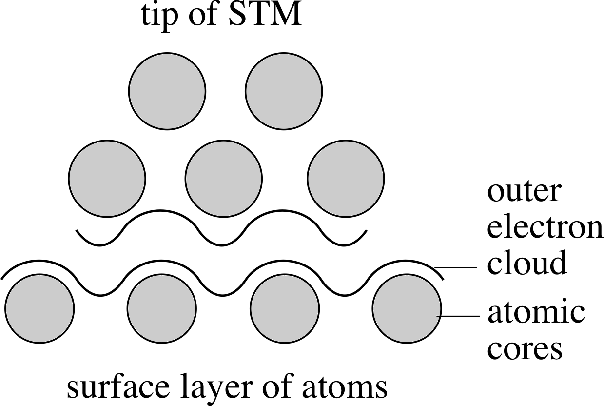
Figure 4 A schematic diagram of a scanning tunnelling microscope.
A much more modern development is the scanning tunnelling microscope, or STM. Dating from 1982, this instrument can be used to obtain direct information about the vertical profile of electrically conducting surfaces, with a resolution of better than 0.01 nm. A schematic of the essential parts of such a microscope is shown in Figure 4.
Although the physical principles of the STM are firmly based in quantum physics, we can very crudely picture its operation as follows. The primary feature of the STM is a sharpened metallic tip, much sharper than a needle, tapering to a span of a few atoms. A voltage difference is maintained between the tip and the surface of the material being studied. When the tip is brought close enough to the surface, electrons can move across from the tip to the surface, forming a small current. (This movement of electrons is known as quantum_tunnellingtunnelling in quantum physics, hence the name of the instrument.) i The magnitude of this current depends very sensitively on the distance between the tip and surface, dropping exponential_functionexponentially as the distance increases. (This also serves to make the effective tip area even smaller. It is only the nearest atoms on the tip which contribute to the current.) i
Question T7
The dependence of the tunnelling current I on the distance L between the tip and the surface can be described approximately by the expression I = I0 exp(−2L/δ), where δ is approximately 0.1 nm.
(a) If the measuring device can detect a current change of 2%, what change in L will be detectable?
(b) The diameter of an atom can be taken to be approximately 0.3 nm. What will be the fractional reduction in the current passing to a part of the tip that is an atomic diameter further away?
Answer T7
(a) The expression I = I0 exp(−2L/δ) can be rearranged to give:
L = −(δ/2) loge (I/I0)
If I changes by 2%, the new separation L′ can be found as:
L′ = −(δ/2) loge (1.02 I/I0) = −(δ/2) [loge (1.02) + loge (I/I0)]
and therefore
∆L = L − L′ = (δ/2) loge (1.02) = 1 × 10⁻³ nm
(b) If L increases by 0.3 nm, then I will be reduced by a factor of
I′/I = exp(−2∆L/δ) = exp(−2 × 0.3 nm/0.1 nm) = exp(−6) = 2.5×10⁻³
i.e. a fractional reduction of 99.75%.
In principle, as the tip of the STM is moved across the surface being studied, changes in the distance between the tip and the surface could be calculated from the measured variations in current. However in practice the current is maintained at a constant value by raising the tip up and down as it moves across the surface. (The feedback and control mechanisms which make this possible are fascinating, but irrelevant to our discussion here.) In a simple case, where only one type of surface atom is involved, the up and down motion of the tip precisely tracks the variations in the height of the surface features of the sample, on a length scale parallel to the surface of about 0.2 nm. The tip can then be moved in parallel tracks across the surface of the sample, determining a series of one–dimensional height profiles which can be put together to form a three–dimensional map of the surface of the sample.
Even more recently developed, the atomic force microscope, or AFM, is similar to the STM, but can be used even when the surface is non-conducting, thus greatly extending the range of materials that can be studied. Instead of a metallic tip, the tip of an AFM is made of a tiny sliver of diamond. Diamond is an electrical insulator, so electrons will not transfer very easily between the tip and surface. Instead, it simply experiences a repulsive force when it gets too close to the surface. By measuring this repulsive force and using feedback and control circuits similar to the STM, a fixed distance can be maintained between the tip and the surface. Thus, again the profile of the surface on an atomic scale can be produced.
In the future, these tools for observing surfaces will certainly be adapted to actually manipulate surfaces at the atomic level. This has already been done in the laboratory, but it may soon become a routine tool for storage of information at the atomic level.
4 Atoms, molecules and matter
4.1 Atoms and molecules: sizes and structures
The most important aspect of atoms and molecules, and one which made it so difficult to form an accurate idea of their existence and properties, is the scale on which they exist. We are used to dealing with objects that are comparable to our own size, in other words, on a length scale from metres down to millimetres. As mentioned in the previous section, the optical microscope gave us access to length scales which were a thousand times smaller, on the order of micrometres (or microns). Yet, even in this microscopic world, matter is essentially continuous. To ‘see’ the basic constituents of matter, we need instruments such as the electron microscope or the scanning tunnelling microscope that can probe matter on a scale which is a thousand times finer still. It is likely that such sizes, on a length scale of nanometres, are beyond our capacity for direct visualization. One consequence of this tiny scale is that the numbers of atoms and molecules contained in everyday objects are huge, as expressed by the magnitude of Avogadro’s constant.
The earliest models of atoms treated them simply as very small hard spheres, which acted upon each other only through direct contact. This was sufficient to provide the basis for the earliest versions of kinetic theory, which sought to explain the properties of gases. However, towards the end of the 19th century, the discovery of the electron and measurements of the spectral lines emitted by excited atoms led to the realization that the supposedly indivisible atom must, in fact, be quite a complicated structure.
The earliest structural models for atoms in the twentieth century tried to reconcile experimental observations of the structure and properties of atoms with the tenets of classical physics. This led to models such as J. J. Thomson’s i plum–pudding model, which had electrons embedded in symmetric positions in an extended sphere of positive charge. It was hoped that frequencies of oscillation of the electrons about their assumed equilibrium positions would correspond to the observed frequencies of the emitted spectral lines. i
The experimental observations of Rutherford i on alpha_particleα–particle (alpha-particle) scattering from thin gold foils showed that the Thomson plum–pudding model wasn’t good enough. When α–particles were directed at the gold foil, a definite fraction of them were scattered at large angles out of the foil, rather than suffering only minor deflections. Some of the α–particles were even scattered backwards, retracing their original paths, with almost no loss in speed; this meant that there had to be a dense lump in the atom which was much more massive than the scattered α–particle.
Question T8
From the theory of collisions in mechanics, it is known that for a one–dimensional collision between a particle of mass m1 and a stationary target particle of mass m2, the final velocity υx(f) of the first particle can be expressed in terms of the two masses and its initial velocity υx(i) as:
$\upsilon_x({\rm f}) = \left(\dfrac{m_1-m_2}{m_1+m_2}\right)\upsilon_x({\rm i})$
In the one–dimensional case, the α–particle scattering described above can be thought of as the first particle travelling along the x–axis and rebounding backwards with almost its initial speed. Show how the collision equation above implies that the target particle’s mass must be much larger than the α–particle’s mass.
Answer T8
The result of the experiment is essentially that υx(f) = −υx(i). This requires that (m1 − m2) ≈ − (m1 + m2) which means that 2m1 ≈ 0, which we have to interpret as m2 ≫ m1.
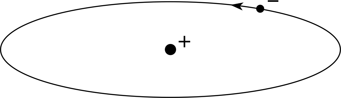
Figure 5 The planetary model of the atom, which can illustrate both the Rutherford and Bohr theories.
This experimental result led to the ascendancy of the nuclear model of the atom, with the positive charge being localized in the centre of the atom and the electrons circling it in motions that closely resembled the motion of the planets around the sun. This is illustrated in Figure 5.
Unfortunately, the nuclear model of the atom was also unstable according to classical theories of electromagnetism, because the electrons in orbit should have radiated their energy away continuously. Furthermore, the protons in the central nucleus should have been driven apart by electrostatic repulsion.
The only explanation available at the time was that the nucleus consisted of both protons and electrons, but with more protons than electrons. It left open the question of why some electrons were in the nucleus, while others orbited at comparatively large distances. Rutherford understood these objections, but gave priority to the experimental observation rather than electromagnetic theory. It was assumed that further experiments would explain these apparent anomalies.
In 1913, Niels Bohr i introduced his own model of the atom, which was based on Rutherford’s picture of a miniature solar system, but with some special refinements. Bohr placed non–classical (quantum) constraints on the motion of bound electrons, leading to a definite set of allowed orbits, each with a definite total energy, the outer orbits having higher energies than the inner ones. When an electron was in such an orbit, Bohr further asserted that no radiation would be emitted; radiation was produced when an electron made a transition from a higher orbit to a lower one. With the electrons in their lowest possible orbits, no radiation could be produced so the stability problem was avoided, albeit at the cost of an artificial and unexplained assumption.
The Bohr model was certainly seen as a major advance, largely because it was able to explain many experimental facts, including the wavelengths of the spectral lines emitted by a hydrogen atom. In spite of these successes, however, the Bohr model is no longer taken seriously. It is sometimes used figuratively, as a sort of cartoon, but the modern theory of atoms is based on a far more fundamental revision of classical ideas.
The final theoretical step toward our current model of the atom was taken between 1924–1927. At a rapid pace, de Brogliei introduced the idea of the wave behaviour of electrons, Heisenberg i developed the abstract matrix mechanics and the uncertainty principle, and Schrödinger i developed the more intuitive wave mechanics. The final piece of the puzzle was put into place when Born i arrived at a probability interpretation of the wavefunction.
The complete theory made possible by these advances is now known as (non-relativistic) quantum mechanics.
The final experimental step was the discovery of the neutron by Chadwick i in 1932, although he was reluctant to identify it as a new elementary particle. This then allowed the theorists to dispense with the messy and ad hoc collection of protons and electrons in the nucleus.
Our current model of the atom has the nucleus consisting of protons and neutrons (bound by the non–classical strong_interactionnuclear strong force), with an approximate radius of 10−14 m, which is surrounded by a cloud of electrons whose position is indefinite, but which extends out about 10−10 m from the nucleus. The electrons have neither definite positions nor definite velocities, but it is possible for an electron to have a definite total energy and definite angular momentum magnitude. The quantum picture of an atom replaces the allowed Bohr orbits by allowed quantum states. The quantum states are characterized by discrete, definite values for the energy and angular momentum, but have rather fuzzy locations and velocities for the electrons. As an echo of the Bohr model, the quantum states of higher total energy tend to spread out further from the nucleus. For this reason, the most energetic electrons in an atom are said to form the outer shell while electrons in states of lower energy occupy inner shells.
A chemical element is uniquely characterized by the number of protons in the nucleus (known as the atomic number, Z), which in turn determines the total number of electrons. Modern theories show that the chemical behaviour is determined almost entirely by the number of the electrons surrounding the atomic nucleus and the quantum states they occupy. Each chemical element can however be represented by more than one nucleus; nuclear stability allows for the presence of a variable number of neutrons in the nucleus, which affects the atomic mass without significantly changing the chemical properties. Nuclei which have the same number of protons, but differing number of neutrons, are known as isotopes.
✦ What can you deduce about the relative atomic mass of different isotopes of the same element?
✧ Since an element must have a specified number of protons (and electrons), the difference in the number of neutrons for different isotopes means that the mass of the isotopic nuclei will be different. Therefore the relative atomic mass of different isotopes will be different as well.
The detailed understanding of the structure of complicated atoms and molecules and their interactions requires calculations using quantum mechanics, but these are in general too difficult to be carried out exactly for any but the simplest cases. Instead, it is customary to fall back on modelling these complicated interactions as traditional forces that have some form of distance dependence and depend on some phenomenological parameters. We will discuss these further in the next subsection.
4.2 Types of bonding: how atoms and molecules stick together
Study comment The concepts in this section involve some rather advanced ideas, some of which are covered more fully in other parts of FLAP. Don’t be concerned about a detailed understanding, just try to form a picture of how the bonding mechanisms vary.
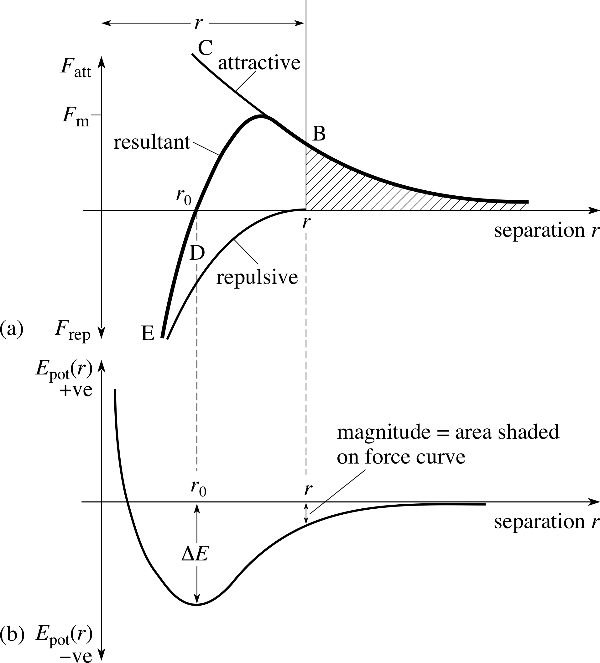
Figure 6 Typical variation of (a) the interatomic force and (b) the corresponding potential energy for two atoms separated by a distance r. When the atoms are very close together there is a repulsive force (as at point E), when they are further apart the force is attractive (as at B).
The types of bonding between atoms and molecules that are responsible for the properties of matter are ultimately based on quantum mechanics as well as electrostatic forces. The electrostatic forces primarily act between the electron clouds of the outer shells of the atom (known as the valence electrons), and depend on the detailed spatial distribution of the electron densities. In addition to the classical electrostatic force, there are important restrictions on the quantum states that electrons are allowed to occupy, through the mechanism known as the Pauli exclusion principle. i Briefly, this principle states that two identical particles (such as two electrons) cannot be in the same quantum state. Under some circumstances, the exclusion principle places restrictions on how particles can move, in the same way that classical forces in physics affect the way particles move. This effect can be pictured as a new, non–classical repulsive force called the quantum exchange force. Thus, the Pauli exclusion principle leads to an effective repulsive force between electrons, and hence between atoms. It is the combination of this quantum force with the electrostatic force which is responsible for atomic interactions.
A typical form of the force between two atoms is shown in Figure 6. The essential characteristics of this force are that at large distances it is attractive, tending to pull atoms together, while at small distances it is repulsive, tending to push them apart.
The detailed understanding of these bonds requires a deep understanding of these topics, which are studied in somewhat more detail elsewhere in FLAP. Here we will pursue only a qualitative understanding of these forces, which will help us to understand the varieties of matter and its phases.
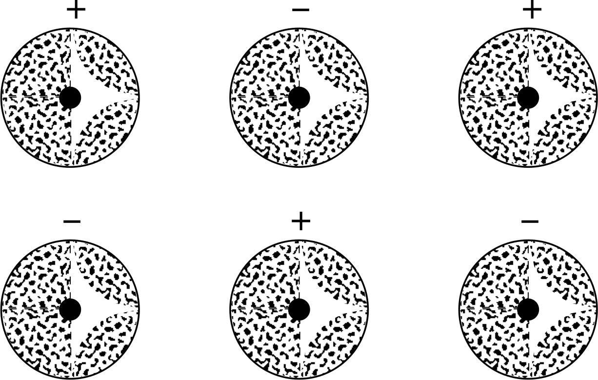
Figure 7 A model for ionic bonding between atoms, illustrating the positive and negative ions bound by the electrostatic force between them.
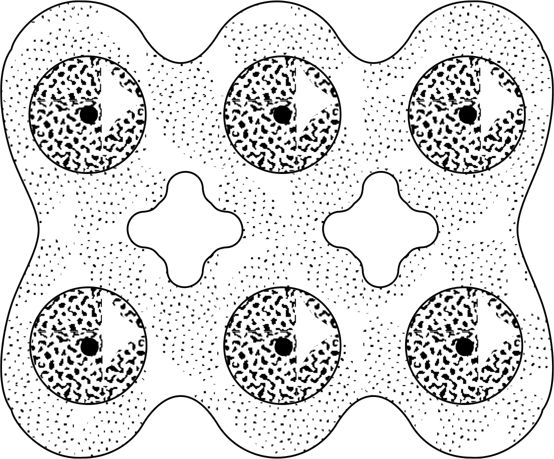
Figure 8 An illustration of covalent bonding between atoms, the result of sharing of electrons between two atoms.
In all cases, the length scales of the interactions can be inferred from our experimental knowledge of the spacing of atoms in physical systems. To characterize the different forms of the bonding interactions, we use the degree of directionality and the energy of the resulting stable equilibrium state ∆E, often measured in electronvolts. i (The electronvolt is of a convenient size to describe energies at the atomic level.) By directionality, we mean that the exact form of the force curve between the atoms or molecules will vary depending on the angle at which they approach each other. This can be understood crudely because the electron clouds have a distinctive shape, which isn’t necessarily spherical.
Pure ionic bonding (illustrated in Figure 7) involves atoms which actually transfer one or more electrons from one to the other, forming a pair of positive and negative ions. These can then be pictured as interacting through the classical electrostatic force. This form of bonding is comparatively non-directional, and has a typical magnitude of 1–5 eV.
Covalent bonding involves the sharing of electrons between atoms, and can be pictured as a state in which the electronic density is higher between the two atoms involved (shown schematically in Figure 8) than would be the case if they were treated as isolated spheres. The cores are positive and are attracted to the electron cloud, which provides the effective force between the atoms. Covalent bonding is characterized by high directionality and a typical magnitude of 1–5 eV.
Metallic bonding only properly occurs in condensed systems with many atoms, and represents a sharing out of electrons into a sea of conducting electrons that belong to no individual nuclei. It can be regarded in a sense as a limiting case of the covalent bond, is non-directional, and has a typical magnitude of 0.2−2eV.
Hydrogen bonding results when a hydrogen atom is ‘shared’ by two different atoms. The hydrogen atom has only one electron, so it can only form one bond in the usual sense. However, the hydrogen atom is unique in that the positive ion is a bare proton, which allows other atoms to reside very close to it. When a hydrogen atom bonds covalently to another atom (such as oxygen, for instance), the shared electron tends to have a higher probability to be located between the two atoms participating in the covalent bond. This leaves the hydrogen atom appearing as an electric dipole i to a third atom, which can form a weak bond with it.
van der Waals bonding i actually covers a range of bonding mechanisms, all involving electrostatic interactions between electric dipoles, either intrinsic, induced or fluctuating. An electric dipole can be regarded as a sort of dumbbell of equal positive and negative charge separated by some distance. The system will be electrically neutral overall, but can still interact electrically with other electrical systems. A fluctuating dipole is produced by time–dependent variations in the shape of the electron cloud of an atom. This dipole creates an electric field which induces a dipole in neighbouring atoms. It is the interaction between these fluctuating induced dipoles that produces a small attractive force between atoms. Because of the overall electrical balance, the energy of van der Waals bonds tends to be substantially lower, on the order of 0.1–0.2 eV. They also tend to be fairly non-directional.
Note that all the types of bonding mentioned above are simply categories which are not totally distinct, but represent idealized models. In real systems, these different effects merge into a continuum of bonding behaviour, with particular systems being closer to one model rather than another.
4.3 Gases, liquids and solids: three phases of matter
Study comment We will present concepts in this section that are elaborated in other modules in this block. Don’t worry if your understanding is a bit vague, because the intention here is to establish a general perspective of these ideas.
You will be familiar with the three ordinary phases of matter, by which we mean the forms that matter takes, each of which has its own distinctive properties. These three normal phases are gas, liquid and solid, and are exemplified by our everyday experience with steam, liquid water, and ice. We now want to characterize the macroscopic differences between these phases more carefully, and try to understand what they imply about the microscopic states of matter in these phases.
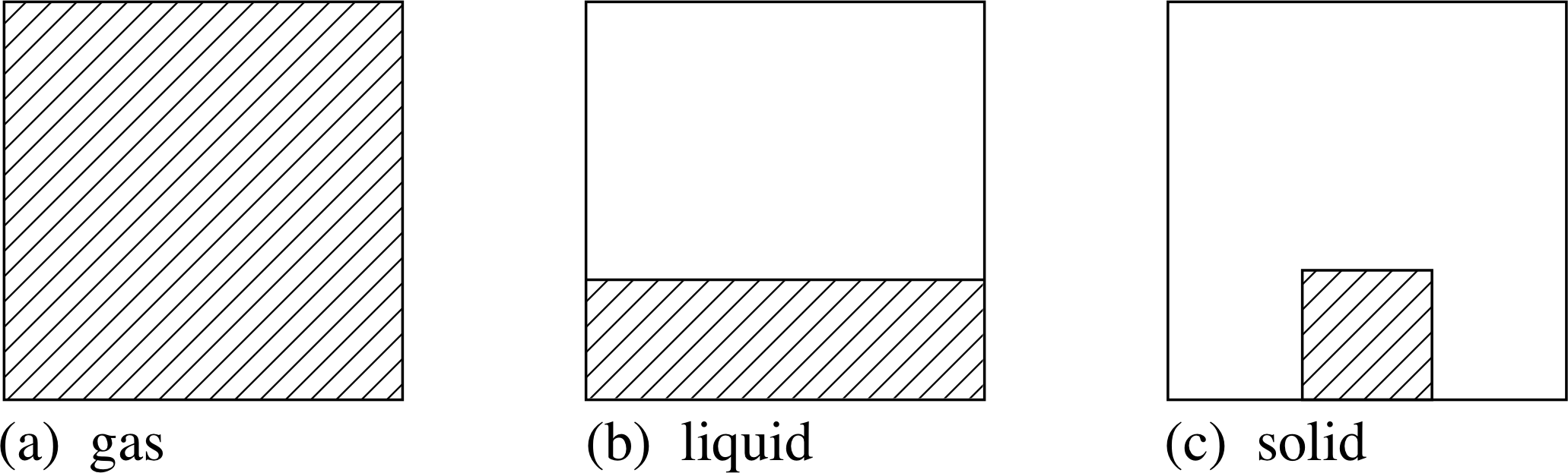
Figure 9 Model of the macroscopic physical state of a gas, liquid
In everyday experience, a gas is characterized by low density, fluidity, and the fact that it fills any container, adopting both the shape and volume of the container (Figure 9). It is also true that, for normal temperatures and pressures, a gas is rather easily compressed.
A liquid is also a fluid, but typically has a much higher density than a gas. It still adopts the shape of its container, but the most significant difference is that the liquid has a definite volume, and resists compression more strongly.
Finally, a solid has a somewhat higher density, but is essentially distinguished by its rigidity, so that it tends to maintain both a definite volume and a definite shape.
It must be admitted that these distinctions between the different phases of matter are not always clear-cut. A gas can be pressurized and made more dense so that it becomes viscous, like a liquid. Solids can sometimes flow very slowly, as you can see from the distorted shapes of some very old stained glass windows. Nevertheless, the distinction between gases, liquids and solids is usually obvious enough, especially when there are clear transitions from one phase to another, as when ice melts or water boils.
In approaching the understanding of these different phases of matter, it is important to remember the modern point of view that all three consist of the same basic atoms or molecules. This is made more plausible when we recall that the three phases can be transformed into each other by appropriate changes in their temperature or pressure. We want to understand the phases in terms of a balance between the forces that act between the atoms (based qualitatively on the typical force curve in Figure 7) and their kinetic energies. As the temperature of a substance is raised, so the average kinetic energy of its atoms or molecules increases. It is no accident that solids form at low temperature, liquids at higher temperature and gases at higher temperatures still; the increase in temperature corresponds to giving the atoms in the substance more kinetic energy, allowing them progressively to escape from the confining attraction of the interatomic forces.
Let us start with the gas phase which is found at high temperatures. This has the lowest density, which implies that the atoms are farthest apart from each other. In terms of our force curve, this means that the force experienced on average is a small attractive force, but generally so small that we can treat the atoms as having no force acting between them most of the time. Only very occasionally do atoms come close enough together to experience a strong repulsion; they then collide rather like billiard balls, exactly as assumed in the classical kinetic theory of gases. Ignoring the small effects of gravity, the molecules in a gas can be thought of as undergoing high–speed straight–line motions, punctuated by random collisions with other molecules and collisions with the walls of the container.
A liquid can be produced by cooling a gas. The reduction in temperature corresponds to a reduction in kinetic energy of the atoms or molecules, until there comes a point where colliding molecules do not necessarily separate after a collision; for technical reasons (related to conservation laws) this requires collisions between more than two molecules, but once the condensation process has started it gains pace and a liquid phase is rapidly formed. A second way of producing a liquid from a gas is by compression. As one compresses the gas the average distance between the molecules gets smaller, until the distance is such that on average, the molecules are in the region of the force curve corresponding to strong attractive forces. If the temperature is not too high, the gas will then liquefy. Over a short interval of time, a typical molecule in the liquid agitates to and fro, as if trapped in a cage formed by its nearest neighbours but, every so often, a molecule escapes and moves to a different part of the liquid. The overall picture is reminiscent of a barn dance in which partners occasionally change group; it is this freedom of molecules to change their neighbours that allows the liquid to flow.
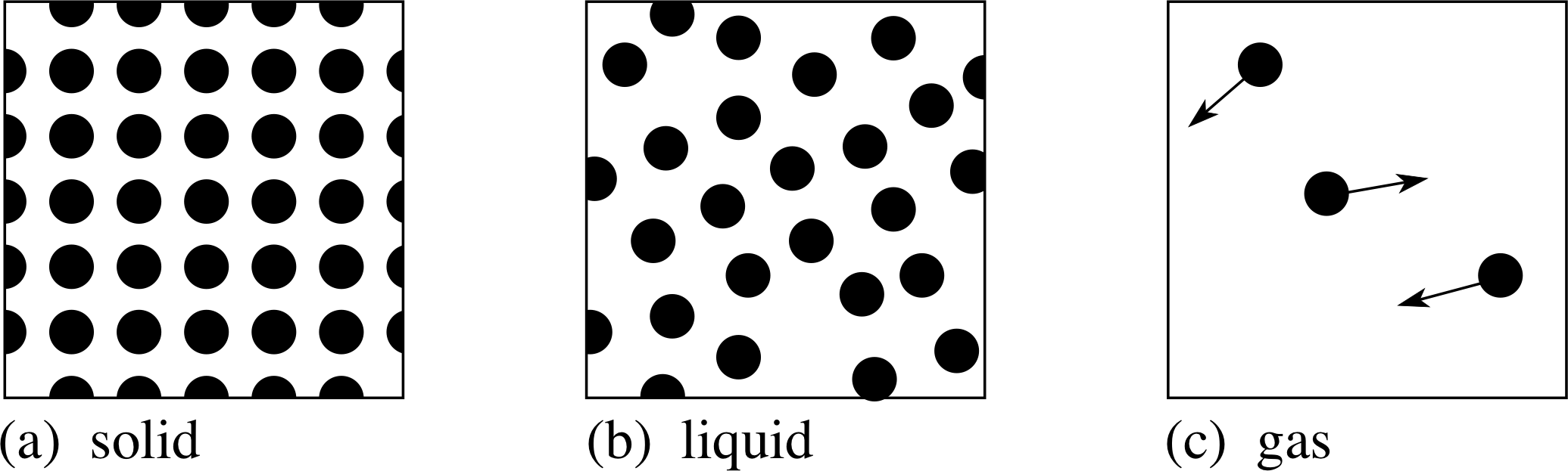
Figure 10 Models of the solid, liquid and gas phases of matter at the atomic level.
Going from the liquid phase to the solid phase, we are primarily removing energy, so that the average speed of the atoms is lower. This means that their motion and position is more tightly constrained by the equilibrium position of the force curve. In a solid the individual atoms oscillate about fixed equilibrium positions, and there is only very limited scope for motion through the solid (diffusion). In a crystalline solid the atoms are tightly regimented into a regular array, quite unlike the more random assemblies in gases, liquids or amorphous solids. Remember, it was the existence of such regular arrangements of atoms that produced sharp spots in an X–ray diffraction pattern and gave good evidence for the existence of atoms in the first place.
Finally, we can schematically represent these three physical states at the atomic level as in Figure 10.
Question T9
For carbon dioxide in the vicinity of 0°C, the gas phase has a density of 11 kg m−3, the liquid phase has a density of 930 kg m−3, and the solid phase has a density of 1500 kg m−3. Assume that one mole of carbon dioxide has a mass of 44 g. From these data, calculate how many carbon dioxide molecules there are per cubic metre in the three phases.
Answer T9
44 g mol−1 can be written as:
22.7 mol kg−1 = 22.7 mol kg−1 × 6.02 × 1023 kg−1 = 1.37 × 1025 molecules kg−1
We now need to multiply this value by the density in the three phases to obtain the number of molecules per cubic metre for each phase. This calculation gives 1.5 × 1026 molecules m−3 in the gas, 1.3 × 1028 molecules m−3 in the liquid, and 2.1 × 1028 molecules m−3 in the solid.
5 Closing items
5.1 Module summary
- 1
-
The concept of atoms has been in existence in one form or another for more than two thousand years, at least since the time of Leucippus and Democritus in the 5th century BC, but for most of that period it had only philosophical significance by modern standards of scientific theories.
- 2
-
Atoms only became a detailed basis for theories of chemistry and physics in the 19th century. Under the lead of Proust, Dalton, Prout, and Avogadro, the idea of atoms as the elementary constituents of elements and of their combination into molecules to form the constituents of compounds led to the understanding of experimental results in chemistry. Physicists such as Daniel Bernoulli, Clausius, Maxwell and Boltzmann developed the kinetic theory of matter, which allowed for the first time the detailed calculation of macroscopic properties of matter on the basis of the behaviour of microscopic entities.
- 3
-
Avogadro presented the hypothesis that equal volumes of gases at a given temperature and pressure held equal numbers of molecules, along with the concept of Avogadro’s constant, which was the number of atoms or molecules in one mole of matter. Although Avogadro couldn’t provide this value, we now know it to be 6.022 169 × 1023 mol−1.
- 4
-
The phenomenon of Brownian motion in the 19th century provided the earliest experimental evidence for the existence of atoms, although it required theoretical substantiation in the 20th century to be finally convincing as a manifestation of the random impacts of submicroscopic particles in the fluid. X–ray diffraction as analysed using Bragg’s law, nλ = 2d sin θ, provided a means of making detailed, if indirect, measurements of atomic positions.
- 5
-
Modern electron and field ion microscopes produce direct images of the surfaces of solids at the atomic level, but the most detail is furnished by the recent developments of scanning tunnelling microscopes and atomic force microscopes, which allow detailed pictures of surfaces to be obtained with resolutions of less than a nanometre. These can also be used for manipulation at the atomic level, allowing for the ultimate in control of structures.
- 6
-
The modern understanding of atomic structure, derived through a combination of experimentation and theoretical calculation, pictures the atom as a quantum–mechanical object constructed from a nucleus with a size on the order of 10−14 m (made up of protons and neutrons) surrounded by a somewhat diffuse cloud of electrons that extends about 5 × 10⁻¹⁰ m from the nucleus.
- 7
-
The forces that bind atoms and molecules are the classical electrostatic force combined with the non–classical quantum exchange force, a consequence of the Pauli exclusion principle. Although the binding can only properly be understood in terms of detailed quantum–mechanical calculations, these are too difficult and complex to allow for easy understanding, and it is customary to model the behaviour in terms of different types of bonds. These range from the ionic bond, which has almost completely localized electrons, through covalent bonds, which have valence electrons shared by atoms, to metallic bonds, which have the valence electrons almost completely delocalized, being shared out among all the atoms in the solid. Hydrogen bonds and van der Waals bonds are weaker mechanisms which come into importance only when the stronger bonding mechanisms are absent.
- 8
-
The standard three phases of matter are the gas, liquid and solid. At the macroscopic level, these differ in their density and rigidity. At the atomic level, these phases can be understood in terms of the balance between atomic and molecular separations and forces and the energy available to the constituent particles.
5.2 Achievements
After completing this module, you should be able to:
- A1
-
Define the terms that are emboldened and flagged in the margins of the module.
- A2
-
Describe the fundamental ideas about the existence of atoms and relate them to chemical and physical principles.
- A3
-
Explain the various forms of experimental evidence for the existence of atoms.
- A4
-
Give the magnitude of the size of atoms, and discuss the experimental evidence that provides these estimates.
- A5
-
Use Bragg’s law to relate the spacing between atomic planes and observed diffraction patterns (in very simple cases).
- A6
-
Discuss qualitatively the various forms of bonding between atoms, and the relationship between these bonding forces and the different macroscopic forms of matter.
Study comment You may now wish to take the following Exit test for this module which tests these Achievements. If you prefer to study the module further before taking this test then return to the topModule contents to review some of the topics.
5.3 Exit test
Study comment Having completed this module, you should be able to answer the following questions each of which tests one or more of the Achievements.
Question E1 (A2)
Explain how Dalton’s concept of the atomic basis of matter and the combination of atoms to form molecules can explain Proust’s law of definite proportions.
Answer E1
According to Dalton’s idea, each compound will be formed from a certain number of atoms of the constituent elements. We can express this by equating the mass of a molecule to the sum of some number of masses of each atom, or mcompound = n1m1 + n2m2. Then any amount of the compound will be some multiple of this mass Nmcompound = Nn1m1 + Nn2m2. The proportion by mass (or weight) of each element in the compound is then just
$\dfrac{Nn_1m_1}{Nn_1m_1 + Nn_2m_2} = \dfrac{n_1m_1}{n_1m_1 + n_2m_2}$
which is independent of N and hence of the total amount of the compound. Thus these proportions are fixed, or definite.
(Reread Subsection 2.1 if you had difficulty with this question.)
Question E2 (A2)
A chemist reports that 1.42 litres of one gas and 2.20 litres of a second gas react completely to form a third gas. Do you think the result is likely to be accurate? Explain your reasoning.
Answer E2
The ratio of these two quantities is 2.20/1.42 = 1.55. If Dalton’s hypothesis is correct, the fraction should be the ratio of two whole numbers. The number is different from 3/2 by 3%, which suggests that the values quoted for the volumes might be inaccurate by approximately this amount.
(Reread Subsection 2.1 if you had difficulty with this question.)
Question E3 (A5)
An experiment in X–ray diffraction using a wavelength of 0.154 nm detects a peak at a Bragg angle of 18°.
(a) If this is the lowest order reflection (n = 1 in Bragg’s law), what is the plane spacing that produces this peak?
(b) At what angles would higher order reflections from this spacing be found?
Answer E3
(a) The spacing in Bragg’s law can be expressed as nλ/(2 sin θ). For n = 1 and λ = 0.154 nm, d = 0.154 nm/(2 sin 18°) = 0.249 nm.
(b) For larger values of n, sin θ = nλ/(2d) = 0.309 n. So θ = arcsin(0.309n) = 38° for n = 2 and 68° for n = 3. Values of n > 3 will not occur.
(Reread Subsection 3.2 if you had difficulty with this question.)
Question E4 (A3 and A4)
Suppose a microscope were designed to use hydrogen ions (i.e. protons) instead of electrons. The proton has a mass of 1.67 × 10⁻²⁷ kg and the electron mass is 9.11 × 10⁻³¹ kg. Assuming the protons and electrons were accelerated to the same speed, what improvement in resolution for the microscope would you expect?
Answer E4
Since the quantum mechanical wavelength depends inversely on the mass, a larger mass implies a smaller wavelength. All other factors being the same, we would expect the improvement in resolution to be equal to the ratio of the masses. Here this is 1.67 × 10⁻²⁷ kg/9.11 × 10−31 kg ≈ 1800, so we would expect the resolution to be 1800 times better.
(Reread Subsection 3.3 if you had difficulty with this question.)
Question E5 (A2 and A4)
Silver has a density of 10.5 g per cubic centimetre.
(a) If its molar mass is 107.9 g per mole, how many silver atoms are there per cubic centimetre?
(b) If you assume that the silver atoms are cubes that completely fill the solid, what would the side of this atomic cube be?
Answer E5
(a) 107.9 g mol−1 can be written as 9.27 mol kg−1 or
9.28 mol kg−1 × 6.02 × 1023 mol−1 = 5.58 × 1024 atoms kg−1
Now 10.5 g cm−3 = 0.0105 kg cm−3, so the number of silver atoms in one cubic centimetre is:
5.58 × 1024 atoms kg−1 × 0.0105 kg cm−3 = 5.86 × 10²² atoms cm−3
(b) The inverse of the answer from (a) is the volume per atom = 1.71 × 10⁻²³ cm3. The cube root of this gives the side of the cubical silver atom, which is 2.57 × 10⁻⁸ cm = 0.257 nm.
(Reread Subsection 2.2 if you had difficulty with this question.)
Question E6 (A2 and A4)
Aluminium and lead have atomic numbers of 13 and 82 and relative atomic masses of 27 and 207, respectively. The respective densities of their solid phases are 2700 kg m−3 and 11 340 kg m−3. These phases have the same sort of crystal structure. What can you conclude about the relative sizes of aluminium and lead atoms (assuming that the atoms are packed tightly together in the solid phase)?
Answer E6
The ratio of their atomic numbers is 6.3 and the ratio of their masses is 7.7. The density ratio is only 4.2, which means that the size of atoms increases more slowly than either the number of protons (or electrons) or than the total mass.
(Reread Subsection 4.3 if you had difficulty with this question.)
Question E7 (A6)
Using the data given in Question T9, calculate the average distances between carbon dioxide molecules in the three phases.
Answer E7
From Question T9 we can say there are 1.5 × 1026 molecules m−3 in the gas, 1.3 × 1028 molecules m−3 in the liquid, and 2.1 × 1028 molecules m−3 in the solid.
The volume per molecule is the inverse of these, i.e. 6.7 × 10⁻²⁷ m3 in the gas, 7.7 × 10⁻²⁹ m3 in the liquid, and 4.8 × 10⁻²⁹ m3 in the solid.
The average distance between molecules will be just the cube root of these numbers. This yields 1.9 × 10⁻⁹ m for the gas, 4.3 × 10⁻¹⁰ m for the liquid, and 3.6 × 10⁻¹⁰ m for the solid, or 1.9 nm, 0.43 nm and 0.36 nm, respectively.
(Reread Subsection 4.3 if you had difficulty with this question.)
Study comment This is the final Exit test question. When you have completed the Exit test go back and try the Subsection 1.2Fast track questions if you have not already done so.
If you have completed both the Fast track questions and the Exit test, then you have finished the module and may leave it here.
Study comment Having seen the Fast track questions you may feel that it would be wiser to follow the normal route through the module and to proceed directly to the following Ready to study? Subsection.
Alternatively, you may still be sufficiently comfortable with the material covered by the module to proceed directly to the Section 5Closing items.