PHYS 7.4: Specific heat, latent heat and entropy |
PPLATO @ | |||||
PPLATO / FLAP (Flexible Learning Approach To Physics) |
||||||
|
1 Opening items
1.1 Module introduction
What happens when a substance is heated? Its temperature may rise; it may melt or evaporate; it may expand and do work – the net effect of the heating depends on the conditions under which the heating takes place. In this module we discuss the heating of solids, liquids and gases under a variety of conditions. We also look more generally at the problem of converting heat into useful work, and the related issue of the irreversibility of many natural processes.
We begin, in Section 2, by defining important some important terms, using them to discuss the heating of solids and liquids, and seeing how the temperature rise of a heated body is related, via the specific heat capacity, to the heat transferred. Next we discuss fusion, vaporization, sublimation and latent heats. We finish the section by outlining some techniques for measuring specific heats and latent heats.
In Section 3 attention turns to gases, where different constraints are readily applied during heating. We deal first with constant volume and constant pressure processes and derive expressions for the corresponding principal specific heats of a monatomic ideal gas. We also investigate the related ratio of specific heats for an ideal gas, and investigate its dependence on the number of atoms in each molecule of a gas, and its role in describing adiabatic processes.
In Section 4 we take a look at phase changes represented on a PVT-surface, and identify the triple point and the critical point.
In Section 5 we introduce the second law of thermodynamics, and show how processes ranging from bench–top experiments to the evolution of the universe can be described in terms of entropy changes.
Study comment Having read the introduction you may feel that you are already familiar with the material covered by this module and that you do not need to study it. If so, try the following Fast track questions. If not, proceed directly to the Subsection 1.3Ready to study? Subsection.
1.2 Fast track questions
Study comment Can you answer the following Fast track questions? If you answer the questions successfully you need only glance through the module before looking at the Subsection 6.1Module summary and the Subsection 6.2Achievements. If you are sure that you can meet each of these achievements, try the Subsection 6.3Exit test. If you have difficulty with only one or two of the questions you should follow the guidance given in the answers and read the relevant parts of the module. However, if you have difficulty with more than two of the Exit questions you are strongly advised to study the whole module.
Question F1
(a) What mass of iron at 17 °C, if dropped into liquid oxygen at its boiling point of −183 °C, will cause 3 g of liquid oxygen to evaporate?
Specific heat of iron = 400 J kg−1 K−1
Specific latent heat of vaporization of liquid oxygen = 2.1 × 10⁵ J kg−1
Answer F1
The iron, mass m, cools to −183 °C so its temperature change ∆T/K = ∆T/°C = 17 + 183 = 200. Assuming that heat is transferred only from the iron to the liquid oxygen, then
heat lost by iron = heat used to evaporate 3 g of oxygen at 17 °C
Therefore,
m × 400 J kg−1 K−1 × 200 K = 3 × 10−3 kg × 2.1 × 102 J kg−1
and hence m = 7.9 × 10⁻³ kg = 7.9 g
Question F2
A sample of n moles of an ideal monatomic gas initially at pressure P1, volume V1 and temperature T1, undergoes a change to a final state with pressure 2P1 and volume 2V1. Show the initial and final states, and their temperatures, on a P–V diagram. Suppose you calculated the entropy change involved in this process when the change is brought about (a) by first doubling the volume at constant temperature and then raising the temperature at constant volume, and (b) by an adiabatic rise in pressure from P1 to 2P1 followed by a change of temperature at constant pressure. Why should your answer be the same in both cases?
Answer F2
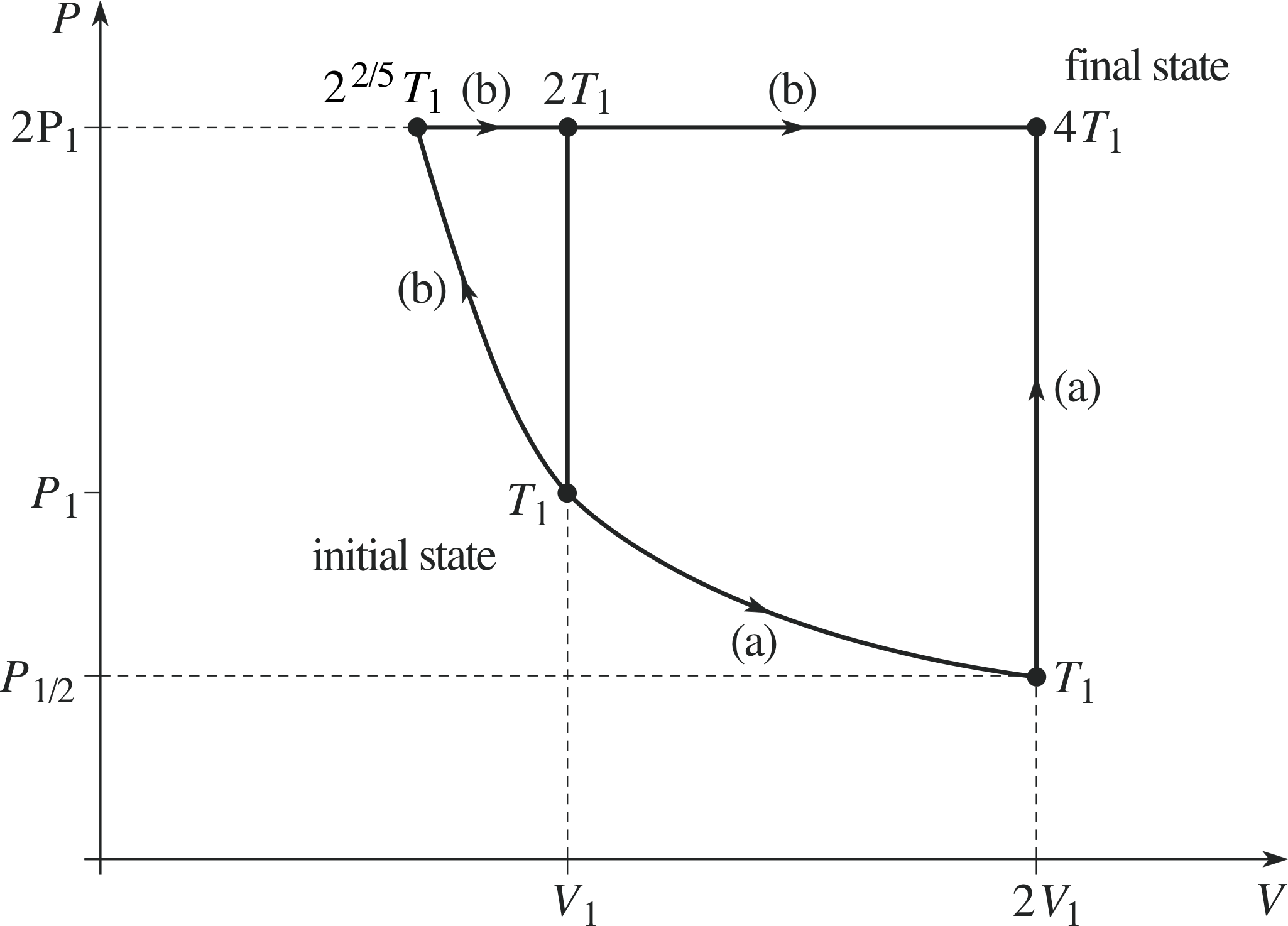
Figure 17 See Answer F2.
The P–V diagram is given in Figure 17. For an ideal gas, PV/T is constant, so the final temperature is 4T1.
Both the given processes, and any others you care to invent, give the same answer because entropy is a function of state, i.e. it depends only on pressure and volume. The explicit demonstration that this is so in this case is given below, but you were not required to carry out this calculation.
(a) V1 to 2V1 at constant temperature T1 (pressure decreases from P1 to ½ P1) followed by ½ P1 to 2P1 at constant volume (temperature increases from T1 to 4T1). In the first part, because the internal energy is unchanged in an isothermal process for an ideal gas, the heat input is equal to the work done,
i.e.$\displaystyle \int_{\rm i}^{\rm f}P\,dV = nRT_1\int_{V_1}^{2V_1}\dfrac{dV}{V} = nRT_1\loge 2$
giving an entropy increase of nR loge 2. The second part is at constant volume 2V1 so the entropy change is
$\displaystyle C_V\int_{T_1}^{4T_1}\dfrac{dT}{T} = \dfrac32nR\loge 2$
The total is thus $nR\loge 2 + \dfrac32nR\loge 4 = nR\loge 2 + 3nR\loge 2 = 4nR\loge 2$
(b) The adiabatic rise in pressure from P1 to 2P1 has zero entropy change but decreases the volume from V1 to $\dfrac{V_1}{2^{1/\gamma}} = \dfrac{V_1}{2^{3/5}}$ and the temperature increases from T1 to 22/5T1. The entropy change all occurs in the second, isobaric, process:
$\displaystyle C_P\int_{2^{2/5}T_1}^{4T_1}\dfrac{dT}{T} = \dfrac52nR\loge\left(\dfrac{4}{2^{2/5}}\right) = \dfrac52nR\loge(2^{8/5}) = 4nR\loge 2$
1.3 Ready to study?
Study comment To begin the study of this module you will need to be familiar with the following terms: energy, kelvin, mole, power, pressure, itemperature, volume and work. It would also be helpful if you have some understanding of the following terms equation of state (of an ideal gas), first law of thermodynamics, function of state, heat, ideal gas, internal energy, quasistatic process and thermal equilibrium. The terms in this second list are introduced in this module, but they are also introduced elsewhere in FLAP, and the treatment here is deliberately brief. If you are uncertain about any of these terms, particularly those in the first list, then you can review them now by referring to the Glossary, which will also indicate where in FLAP they are developed. As well as requiring algebraic manipulation, this module uses the notation of differentiation and integration. You will not be required to evaluate integrals yourself but you will encounter results expressed in terms of integrals and you will be shown (and asked to use) examples in which integrals are evaluated for you. Obviously, the more familiar you are with integration, the easier you will find this material. You will also need to be familiar with the exponential function and with the properties of logarithmic functions. The following Ready to study questions will allow you to establish whether you need to review some of the topics before embarking on this module.
Question R1
Express a temperature of −20 °C as an absolute temperature in kelvin.
Answer R1
T/K = T/°C + 273.15, so to three significant figures, −20 °C is equivalent to 253 K.
(For details about absolute temperature see the Glossary.)
Question R2
Simplify the expression loge (a/b) − loge (c/a).
Answer R2
loge (a/b) − loge (c/a) = loge (a/b) + loge [(c/a)−1] = loge [(a/b)(c/a)−1] = loge (a2/bc)
(For details about logarithmic functions see the Glossary.)
2 Heating solids and liquids
2.1 Heat, work and internal energy
Study comment All of the topics introduced in this subsection are discussed in more detail elsewhere in FLAP. See the Glossary for references to those fuller discussions if you need them.
Solids and liquids are composed of atoms and molecules. These microscopic constituents of matter interact with one another electrically and have some freedom to move, though the movements are very restricted in the case of a solid. As a result of these internal interactions and movements, macroscopic bodies have an internal energy U that can be distinguished from any kinetic_energykinetic or potential energy they may have arising from their overall motion or their interaction with other macroscopic bodies.
The internal energy of a body is a function of state. That is to say, if the body in question is kept under well controlled conditions of temperature and pressure, then its internal energy will be determined by the current values of those conditions.
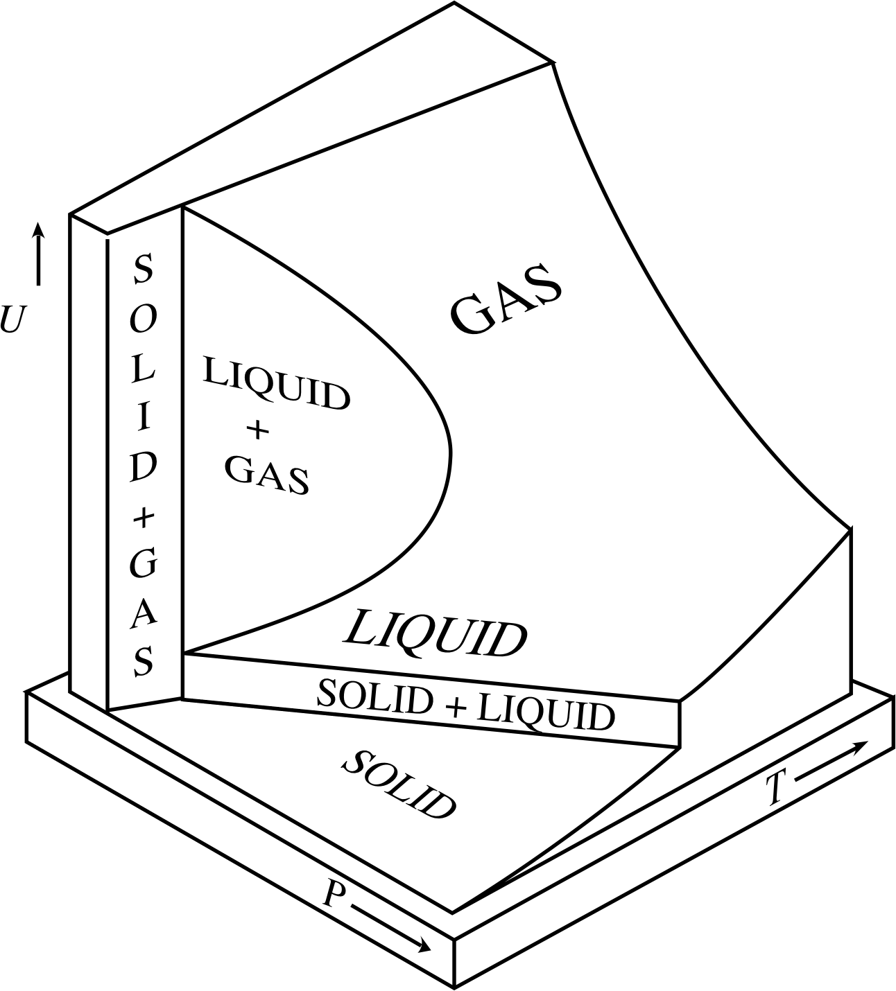
Figure 1 The variation with temperature and pressure of the internal energy U of a fixed quantity of a typical substance. Note that there are vertical regions on the UPT surface (corresponding to changes of phase) in which a change in internal energy is not necessarily accompanied by a change in temperature.
This is indicated in Figure 1, which shows the variation of internal energy with temperature and pressure for a fixed quantity of a typical pure substance. Each point on the two–dimensional internal energy surface relates a value of U to particular values of the pressure P and the temperature T. As you can see, as T increases the surface generally slopes upwards, so there is an overall tendency for internal energy to increase with increasing temperature. However, the relationship is not a simple one, because there are also vertical regions of the UPT surface where the internal energy increases without any corresponding increase in the temperature. These regions correspond to phase transitions, such as melting or boiling, in which the substance changes from one phase of matter (solid, liquid or gas) to another. On the whole, the internal energy of a solid is low, that of a liquid is higher, and that of a gas higher still. If the pressure is held constant during a phase transition there will be no change in temperature while the transition takes place, but the proportion of the more energetic phase will increase as the internal energy increases.
Since energy is a conserved quantity, the only way to alter the internal energy of a body is to transfer some energy to or from that body. There are two ways in which this can be done, the first is to put the body in thermal contact with some other body (or bodies) at a different temperature so that heat can flow from the hotter to the cooler body. Heat is defined as energy transferred due to temperature differences, so the emission or absorption of heat by a body will certainly change its internal energy. The second way of changing the internal energy is to do some work on the body or allow it to do some work. Work is generally defined as energy transfer by any means that does not directly involve temperature differences so it includes processes such as stirring and rubbing which are well known ways of raising the temperature of a body (and hence increasing its internal energy) without having to supply any heat to that body.
The possibility of the internal energy of a body being changed by means of heat or work may be summarized by the equation
∆U = ∆Q − ∆W(1) i
where ∆U is the change in internal energy, ∆Q is the heat transferred to the body, and ∆W is the work done by the body. You may be surprised that we allow ∆W to represent the work done by the body, which will tend to reduce its internal energy, rather than the work done on the body which would increase it.
However, this is a purely conventional choice; the important thing to remember is that any of these quantities may be positive or negative, but with the particular choices we have made:
- A positive value of ∆U implies an increase in internal energy.
- A positive value of ∆Q implies heat transfers energy to the body.
- A positive value of ∆W implies work transfers energy from the body.
The equation ∆U = ∆Q − ∆W is the mathematical essence of the first law of thermodynamics, the full implications of which are explored elsewhere in FLAP.
2.2 Changes of temperature: specific heat
When you heat something – some soup, for example – you supply it with an amount of heat ∆Q which raises its absolute temperature T by an amount ∆T. The ratio of the heat supplied to the consequent change in temperature is called the heat capacity of whatever is being heated.
Thus, heat capacity = $\dfrac{\Delta Q}{\Delta T}$
Strictly speaking, this quantity represents the average heat capacity over the temperature range concerned, since the heat required to raise the temperature from 300 K to 301 K may differ somewhat from that required to raise the temperature from 320 K to 321 K, but we will ignore such variations for the moment.
The heat supplied ∆Q is a quantity of energy, so it can be measured in joules (J) and ∆T can be measured in kelvin (K) or even °C, since a temperature change of 1 °C is the same as a change of 1 K. It follows that the heat capacity ∆Q/∆T can be expressed in units of J K−1 or J °C−1 with the same numerical value in either case. In this module, we will use J K−1.
When dealing with bodies composed of a single uniform substance, the heat capacity is proportional to the amount of that substance within the body. Under those circumstances it is useful to know the heat capacity per unit mass of the substance. In SI units this quantity will have units of J K−1 kg−1 and is usually called the specific heat of the substance, or sometimes its kilogram specific heat. i We will represent this quantity by a lower case c.
The specific heat c of a substance is its heat capacity per unit mass. It follows that the heat ∆Q required to raise the temperature of a mass m of the substance by an amount ∆T is
∆Q = mc∆T(2)
Sometimes, rather than dealing with a known mass of substance we need to deal with an amount defined in terms of a (large) number of its atoms or molecules. On these occasions it is useful to know the heat capacity per mole of the substance. This is usually referred to as the molar specific heat which has SI units J K−1 mol−1. i We will represent this by an upper case C to distinguish it from the specific heat.
The molar specific heat C of a substance is its heat capacity per mole. It follows that the heat ∆Q required to raise the temperature of n moles of the substance by an amount ∆T is
∆Q = nC∆T(3)
thus$C = \dfrac{\Delta Q}{n\Delta T}$
If we use ∆Qm = ∆Q/n to represent the heat supplied per mole i (measured in units of J mol−1), we can rewrite the last equation as
$C = \dfrac{\Delta Q_{\rm m}}{\Delta T}$
As already noted in the case of heat capacity, the relationship between the heat supplied to a sample of a material and the resulting temperature rise depends on the conditions under which it is heated. Thus both the kilogram specific heat c and the molar specific heat C defined in Equations 2 and 3, respectively, are really averages over specific temperature ranges. Moreover, the first law of thermodynamics written in the form
∆Q = ∆U + ∆W(4)
reminds us that the heat ∆Q supplied to an object may enable it to do work ∆W as well as producing a temperature change associated with a change ∆U in its internal energy. The specific heat therefore depends on the way ∆Q is shared between ∆W and ∆U, i.e. it depends on the extent to which a sample is allowed to expand and do work.
When solids and liquids are heated, they are almost always free to expand into their surroundings, so the most widely used specific heats of solids and liquids are those measured at atmospheric pressure. i In fact, specific heats quoted in data books normally refer to measurements made at standard temperature and pressure, (s.t.p.), which means a pressure of 1.00 atm (= 1.01 × 10⁵ Pa = 1.01 × 10⁵ N m−2) and a temperature of 273.16 K (= 0.00°C). In this module, unless told otherwise, you may always assume that the specific heats of solids and liquids are constant, so variations of c or C with temperature may be ignored. However, you should be aware that investigations into the variation of specific heat with temperature have played an important part in the development of modern physics, even though they won’t be pursued in this module.
Question T1
The heat capacity of a copper kettle of mass 1.60 kg is found to be 606 J K−1. One mole of copper has a mass of 64 g. Find the (kilogram) specific heat c and the molar specific heat C of copper. If 200 J of heat is supplied to a 0.25 kg copper block, what is the final temperature of the block if it was initially at 23.0 °C?
Answer T1
The specific heat of the copper is c = 606 J K−1/1.60 kg = 379 J kg−1 K−1. The molar mass of the copper is 64 g mol−1, i.e. 0.064 kg mol−1, so the molar specific heat is
C = 379 J kg−1× 0.064 kg mol−1 = 24.2 J mol−1 K−1
From Equation 2,
∆Q = mc∆T(Eqn 2)
∆T = ∆Q/mc = 200 J/(0.25 kg × 379 J kg−1 K−1) = 2.11 K = 2.11 °C.
The final temperature is therefore
T = 23.0 °C + 2.11 °C = 25.1 °C
2.3 Changes of phase: latent heat
The melting (technically described as fusion i) of ice into water, and the vaporization of water to form steam, are familiar examples of processes in which a substance undergoes a change of phase (known as the phase transition). Sublimation, in which a solid is converted directly to a gas without passing through a liquid phase, is less familiar from everyday experience although solid carbon dioxide (‘dry ice’) sublimes at room temperature and is often used to produce theatrical special effects. i A striking demonstration of sublimation occurs when the silvery, rather metallic-looking, crystals of the element iodine are heated; they do not melt but give off a surprisingly violet–coloured vapour.
Substances such as chocolate, butter and honey, which are made up of murky mixtures of this and that, may melt over a range of temperatures, but the temperatures at which pure solids melt are extremely narrowly defined. i For example, pure ice melts into water at the very well specified temperature of 0 °C – one microdegree below the melting temperature and it is solid; one microdegree above and it is liquid. For the sake of simplicity we will confine ourselves to such well behaved substances for the rest of this module.
Figure 2 A heating curve for 1 kg of ice, at atmospheric pressure.
Figure 2 shows the temperature of a fixed sample of pure water (H2O) i, initially ice, as it is heated at a constant rate. i Below the melting point the temperature of the ice rises steadily, at a rate determined by its heat capacity. Then, at the melting point (0 °C), the temperature ceases to change, even though heating continues. When all the ice has melted the temperature starts to rise again, but not at the same rate as before, since the heat capacity of the liquid water is different from that of the solid ice. The graph flattens again at the boiling point, as the liquid water turns to steam. Finally, the graph starts to rise again at a rate determined by the heat capacity of the steam. Since heat is being supplied at a constant rate, the lengths of the horizontal portions of the graph are proportional to the amounts of heat required to complete the corresponding phase changes. As you can see they are substantial, especially that for the vaporization of water.
By studying graphs similar to Figure 2, for fixed quantities of material under specified conditions (e.g. constant pressure) it is possible to determine the heat required to produce a given phase transition under given conditions. This is referred to as the latent heat of that transition.
The latent heat of a sample is the heat required to change the phase of the whole sample at constant temperature.
As in the case of heat capacity, it is useful to know two related quantities:
The specific latent heat l of a substance is the latent heat per unit mass of the substance. It follows that the heat ∆Q (supplied at constant temperature) required to change the phase of a mass m of the substance is
∆Q = ml(5)
The molar latent heat L of a substance is the latent heat per mole of the substance. It follows that the heat ∆Q (supplied at constant temperature) required to change the phase of n moles of the substance is
∆Q = nL(6)
✦ What are suitable SI units for latent heat, and for the specific latent heat l and molar latent heat L?
✧ Latent heat has the units of heat, i.e. J. It follows that l has units J kg−1 and L has units J mol−1.
When quoting a value for any specific latent heat it is always important to make clear which phase transition it refers to. This is usually done by attaching appropriate subscripts to the relevant symbol, ‘fus’ for fusion, ‘vap’ for vaporization and ‘sub’ for sublimation. This is indicated in Table 1, which lists some of the thermal properties of H2O.
| Quantity | Value |
|---|---|
| specific latent heat of boiling water, lvap | 2.257 × 10⁶ J kg−1 |
| specific latent heat of melting ice, lfus | 3.33 × 10⁵ J kg−1 |
| specific heat of water, c (at s.t.p.) | 4.2174 × 10³ J kg−1 K−1 |
As with specific heat, the values of latent heat and the temperatures at which a substance melts and boils can depend on external conditions. For example, reducing the external pressure lowers the boiling point of a liquid (loosely speaking, because it becomes ‘easier’ for the molecules to escape from the liquid to the vapour) so tea brewed in an open container on a high mountain top is only lukewarm. Values quoted in tables and data books generally refer to measurements at 1 atm.
Question T2
Some vegetables, of heat capacity 2200 J K−1, at T = 373 K, are plunged into a mixture of 1 kg of ice and 1 kg of water at 273 K. How much ice melts?
Answer T2
We make the working assumption that there is some ice left at the end and that therefore the final temperature is T = 273 K.
The vegetables have ∆T = (373 − 273) K = 100 K, so the heat lost by the vegetables is
2200 J K−1 × 100 K = 2.20 × 10⁵ J
The mass of ice melted is therefore
$\rm \dfrac{2.20\times10^5\,J}{3.33\times10^5\,J\,kg^{-1}} = 0.66\,kg$
(Note that the working assumption has thrown up no problems and has thus been justified.)
Question T3
Steam at 100 °C is passed into a beaker containing 0.020 kg of ice and 0.10 kg of water at 0 °C until all the ice is just melted. How much water is now in the beaker?
Answer T3
The heat required to melt 0.020 kg of ice is 0.020 kg × 3.33 × 103 J kg−1 = 6.66 × 10³ J. Suppose the melting is caused by a mass m of steam condensing (i.e. turning to water) and then cooling by 100 K to 0 °C. Then:
heat lost by steam = m × [2.26 × 10⁶ J kg−1 + (4.22 × 10³ J kg−1 K × 100 K)]
i.e.heat lost by steam = m × 2.68 × 10⁶ J kg−1
Sinceheat lost by steam = heat required to melt ice,
6.66 × 10³ J = m × 2.68 × 10⁶ J kg−1
so,m = 2.5 × 10⁻³ kg
At the end, the total amount of water will be the sum of the original amount (0.10 kg), the melted ice (0.020 kg),
and the condensed steam (2.5 × 10⁻³ kg), i.e. 0.1225 kg in all.
2.4 Measuring specific heats and latent heats
The measurement of heat and its effects is known as calorimetry (literally ‘heat measuring’). The basic method for measuring specific heat is to supply a known amount of heat to a sample and to measure the resulting temperature rise. There are many variations on this basic method; we will only touch briefly on a few representative examples.
In the method of mixtures, the supply of heat is from (or to) a hotter (or colder) object whose heat capacity is already known. The mixing takes place in a calorimeter (a fancy name for a container used in calorimetry); the simplest type of calorimeter is a metal container of known heat capacity, thermally insulated from its surroundings. Assuming that no heat is lost to the surroundings, and that any heat absorbed by the calorimeter is taken into account, the heat supplied to the cold object is equal to that transferred from the hot object.
Example 1
A small object of mass m = 0.26 kg and unknown specific heat c, initially at 100 °C, is placed into a body of liquid with a heat capacity of 1300 J K−1, initially at 20 °C. The final equilibrium temperature is 25 °C. What is the value of c? Ignore any heat that may be absorbed by the vessel containing the liquid.
Solution
To reach thermal equilibrium, the object cools by 75 K, and the liquid is warmed by 5 K, so (assuming there are no heat losses)
heat gained by liquid = 1300 J K−1 × 5 K = 6500 J
heat lost by object = mc × 75 K
As these two values are equal, we can write
mc = 6500 J/75 K = 86.7 J K−1
Thus, c = 86.7 J K−1/0.26 kg = 333 J kg−1 K−1
An electrical method is often used to heat the sample in a calorimetry experiment, since it is relatively straightforward to measure and control the rate at which heat is supplied. i Measuring the corresponding rate of increase of temperature provides another method of determining specific heats. If the heater has power P, and there are no heat losses, then in a time ∆t, the heat supplied is ∆Q = P∆t. i This will cause a sample of mass m and specific heat c to increase its temperature by ∆T where P∆t = mc∆T.
It follows that the rate of change of temperature with time will be
$\dfrac{dT}{dt} = \lim_{\Delta t\to 0}\left(\dfrac{\Delta T}{\Delta t}\right) = \lim_{\Delta t\to 0}\left(\dfrac{P}{mc}\right) = \dfrac{P}{mc}$
Where we have used the fact that P/mc is a constant and is therefore unaffected by the process of taking the limit as ∆t becomes vanishingly small.
Hence$c = \dfrac Pm\left(\dfrac{dT}{dt}\right)^{-1}$(7)
Question T4
An object with an electrical heater and thermometer attached is isolated from its surroundings. The heater power is 24 W, and the temperature of the object rises at a rate of 3 degrees per minute. What is the heat capacity of the object?
Answer T4
dT/dt = 3 K min−1 = 5 × 10⁻² K s−1
Therefore from Equation 7,
$c = \dfrac Pm\left(\dfrac{dT}{dt}\right)^{-1}$(Eqn 7)
The heat capacity is
$mc = \dfrac{24\,{\rm J\,s^{-1}}}{dT/dt} = \rm \dfrac{24\,J\,s^{-1}}{5\times10^{-2}\,K\,s^{-1}} = 480\,J\,K^{-1}$
Question T5
0.20 kg of iron at 100 °C is dropped into 0.090 kg of water at 16 °C inside a calorimeter of mass 0.15 kg and specific heat 800 J kg−1 K−1, also at 16 °C.
Specific heat of iron: 400 J kg−1 K−1
Specific heat of water: 4185 J kg−1 K−1
Find the common final temperature of the water and calorimeter.
Answer T5
Suppose the final temperature of the iron, water and calorimeter is T. Then
heat lost by iron = mc∆T = 0.20 kg × 400 J kg−1 K−1 × (100 °C − T)
and similarly
heat gained by water = 0.090 kg × 4185 J kg−1 K−1 × (T − 16 °C)
andheat gained by calorimeter = 0.15 kg × 800 J kg−1 K−1 × (T − 16 °C)
If no heat is lost from the system, then
0.20 × 400 J K−1 × (100 °C − T) = (0.090 × 4185 + 0.15 × 800) J K−1 × (T − 16 °C)
i.e.80 × (100 °C − T) = (376.65 + 120) × (T − 16 °C)
so8000 °C − 80T = 496.65T − 7946.4 °C
andT = (7946.4 + 8000) °C/(496.65 + 80) = 28 °C (to two significant figures)
Either of the basic methods described above can also be used for fluid i samples, but an alternative is to use a continuous flow method in which the fluid flows at a steady known rate through an insulated tube containing an electrical heater delivering a power P. If in the steady state (not equilibrium) mass flows through the apparatus at a constant rate dm/dt, and shows a constant temperature increase ∆T, then we can say that, in a time ∆t, the mass heated is (dm/dt)∆t, and the energy supplied to that mass is P∆t so (using Equation 2)
$P\Delta t = c\dfrac{dm}{dt}\Delta t\Delta T$(8)
Dividing both sides by ∆t and rearranging gives the specific heat
$c = \dfrac{P}{\Delta T}\left(\dfrac{dm}{dt}\right)^{-1}$(9)
In presenting these methods of measuring specific heat we have made the assumption that heat losses are negligible. In practice this is unlikely to be the case; a great deal of time and effort is spent minimizing heat losses and calculating those which are unavoidable. An advantage of the continuous flow method is that both the heating rate and the flow rate can be altered in such a way that the temperature rise is unchanged. By doing this while assuming that the heat losses are the same it is possible to go a long way towards eliminating them from the final calculation of c. i
Example 2
A liquid flows past an electric heating coil. When the mass flow rate of the liquid is 3.2 × 10⁻³ kg s−1 and the power supplied to the coil is 27.4 W, the inlet and outlet temperatures are 10.4 °C and 13.5 °C respectively. The flow rate is then changed to 2.2 × 10⁻³ kg s−1 and, in order to maintain the same temperatures, the power supplied is adjusted to 19.3 W. Calculate the specific heat of the liquid and the rate of loss of heat.
Solution
We use the following notation: $\dot{Q} = \dfrac{dQ}{dt}$ i is the rate of heat flow from the electrical heater, $\dot{H} = \dfrac{dH}{dt}$ is the rate of loss of heat to the surroundings, $\dot{m} = \dfrac{dm}{dt}$ is the rate of mass flow, ∆T is the difference between the inlet and outlet temperatures, and the required specific heat is c. We can modify Equation 8 to include the heat loss:
$\dot{Q} = \dot{m}c\Delta T + \dot{H}$(10)
We assume that the rate of heat leak $(\dotH)$ will be the same in both cases, so we can write down two simultaneous equations:
$\dot{Q}_1 = \dot{m}_1c\Delta T + \dot{H}\quad\text{and}\quad dot{Q}_2 = \dot{m}_2c\Delta T + \dot{H}$
If we subtract the first equation from the second to eliminate $\dot{H}$ we obtain
$\dot{Q}_2 - \dot{Q}_1 = c\Delta T(\dot{m}_2-\dot{m}_1)$
So,
$c = \dfrac{\dot{Q}_2 - \dot{Q}_1}{\Delta T(\dot{m}_2-\dot{m}_1)} = \rm \dfrac{(27.4−19.3)\,W}{(3.2-2.2)\times10^{-3}\,kg\,s^{-1} \times(13.5-10.4)\,K} = 2.6\,kJ\,kg^{-1}\,K^{-1}$
If we put c into either of the original equations, we find $\dot{H}$. For example
$\dot{H} = \dot{m}_1c\Delta T - \dot{Q}_1$
so$\dot{H} = \rm 27.4\,W - (3.2\times10^{-3}\,kg\,s^{-1}\times2.6\times10^3\,J\,kg^{-1}\,K^{-1}\times3.1\,K)$
i.e.$\dot{H} = \rm 1.6\,W$
To measure latent heat, the methods are essentially very similar to those for specific heats. The basic idea is to supply a known amount of heat at the melting or boiling point and to measure the amount of the substance that changes phase. If you can arrange for two different runs of an experiment to have the same heat losses, you can write down two simultaneous equations and eliminate the heat loss from the calculation.
Figure 2 A heating curve for 1 kg of ice, at atmospheric pressure.
Question T6
Figure 2 refers to 1 kg of H2O electrically heated at a constant rate of 4.0 kW. Using values from the graph, and assuming there are no heat losses, deduce values of the specific latent heat of fusion, lfus, of ice and the specific latent heat of vaporization, lvap, of water.
Answer T6
The melting takes (105 − 25) s = 80 s.
In this time
heat supplied = 4000 J s−1 × 80 s = 3.2 × 10⁵ J
Therefore lfus = 3.2 × 10⁵ J kg−1
The vaporization takes (745 − 205) s = 540 s, during which time the heat supplied is
540 s × 4000 J s−1 = 2.16 × 10⁶ J, solfus = 2.16 × 10⁶ J kg−1.
| Quantity | Value |
|---|---|
| specific latent heat of boiling water, lvap | 2.257 × 10⁶ J kg−1 |
| specific latent heat of melting ice, lfus | 3.33 × 10⁵ J kg−1 |
| specific heat of water, c (at s.t.p.) | 4.2174 × 10³ J kg−1 K−1 |
Comment Given that this is based on values from a graph, these results are in reasonable agreement with the values in Table 1.
Question T7
In measuring the specific latent heat of vaporization of ethanol, a mass of 4.2 g of vapour (gas) was collected in 5.0 min when 4500 J was supplied by an electric heater. In a second run, the heater was adjusted to supply 9000 J in 5.0 min and 9.3 g of vapour was collected. Calculate the specific latent heat of vaporization for ethanol and the heat lost from the apparatus.
Answer T7
Let the heat loss in 5 min be H (it is the same in both runs because the temperature of the sample is the same, namely, the boiling point) and the latent heat l. Then:
for the first run4500 J = 4.2 × 10⁻³ kg × lvap+ H(i)
for the second run9000 J = 9.3 × 10⁻³ kg × lvap+ H(ii)
Subtracting Equation (i) from (ii) eliminates H and gives us
4500 J = (9.3 − 4.2) × 10−3 kg × lvap
hencelvap = 8.82 × 10⁵ J kg−1
If we then substitute lvap into either of the original equations, we find H = 797 J.
3 Heating gases
In this section, we look at processes that involve the heating of gases and the constraints (e.g. maintaining constant pressure or constant volume) that may be applied during such processes. It was noted earlier that such constraints can have a substantial influence on the specific heats of gases. We will begin with a brief review of some key ideas and equations.
3.1 Ideal gases
Study comment All of the topics introduced in this subsection are discussed in more detail elsewhere in FLAP. See the Glossary for references to those fuller discussions if you need them.
Real gases behave in a variety of different ways, but at low density and moderate temperature the behaviour of all real gases approximates the behaviour of an ideal gas. A quantity of n moles of ideal gas at absolute temperature T and pressure P, contained in a volume V satisfies the equation of state of an ideal gas
PV = nRT(11)
where R = 8.314 J K−1 mol−1 is the molar gas constant (T must be expressed in kelvin (K), not °C).
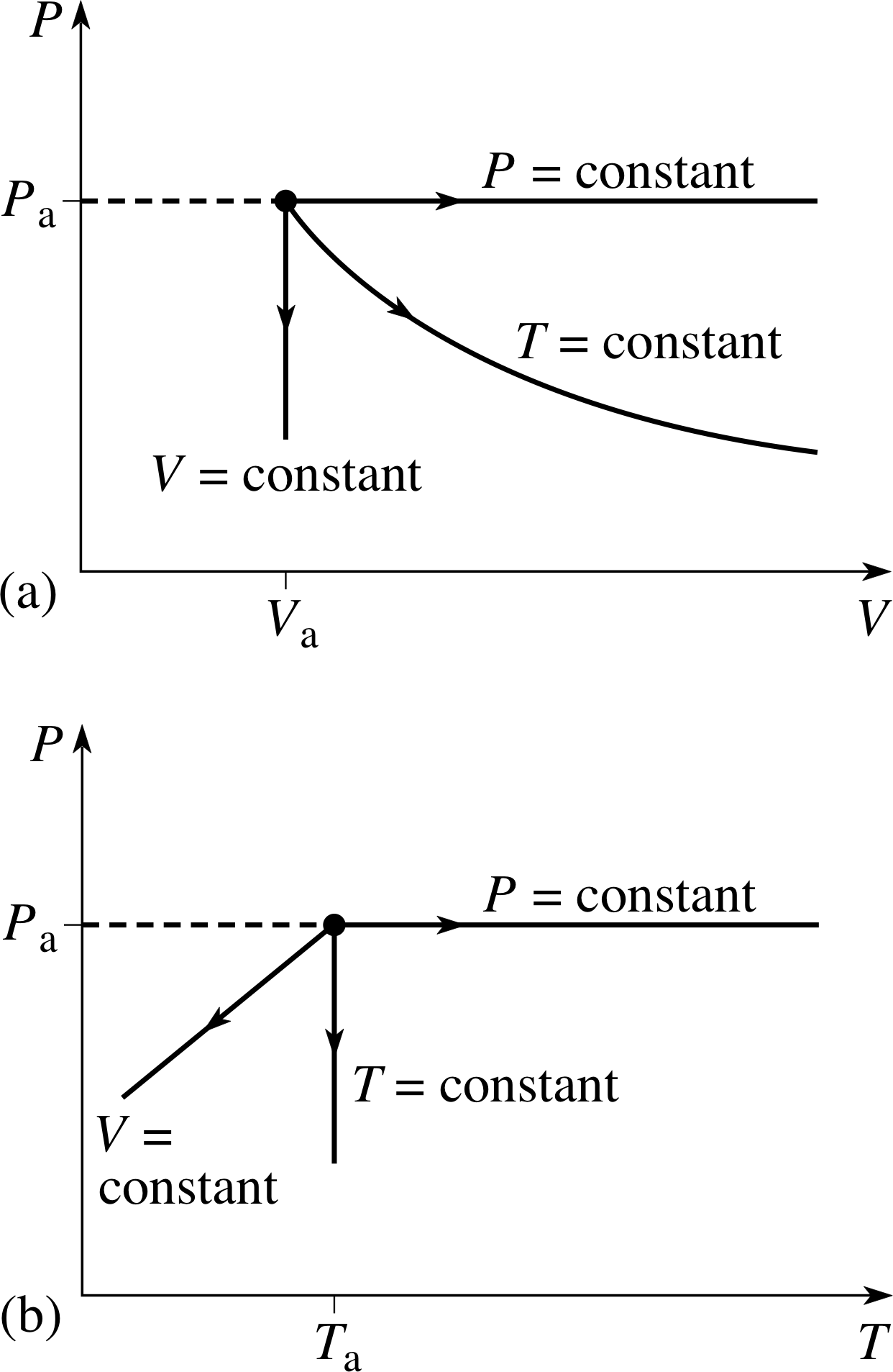
Figure 4 (a) P–V and (b) P–T graphs of three simple quasistatic processes in a fixed quantity of ideal gas which is initially in an equilibrium state specified by pressure Pa, volume Va and temperature Ta. The three processes respectively involve: constant temperature (Ta), constant pressure (Pa) and constant volume (Va).
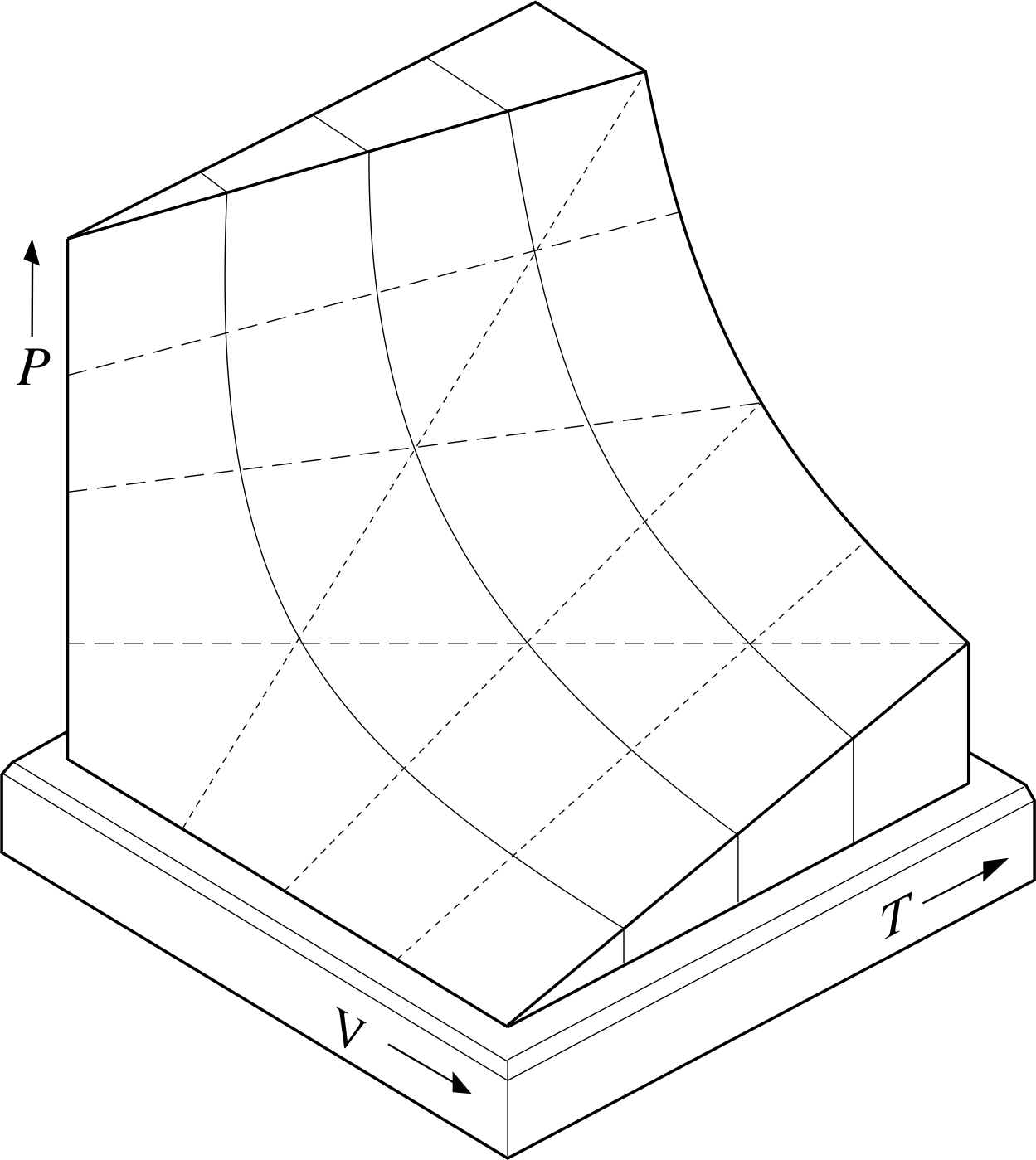
Figure 3 The (truncated) PVT–surface of a fixed quantity of ideal gas, representing its possible equilibrium states. The dashed lines drawn on the surface correspond to constant values of P, the solid lines to constant T, and the dotted lines to constant V.
The relationship between P, V and T given by Equation 11 can be shown graphically by using a three–dimensional graph of the sort shown in Figure 3. For a given value of n (i.e. for a fixed quantity of gas) each set of values for P, V and T that satisfies Equation 11 specifies a single point on the graph and corresponds to a unique equilibrium state of the sample. The set of all such points (i.e. the set of all equilibrium states of the fixed quantity of gas) constitutes a continuous two–dimensional surface in the three–dimensional PVT space of the graph. Such a surface is called the PVT–surface of the gas. The surface shown in Figure 3 has been truncated for ease of display, but ignoring that, every possible equilibrium state of the sample is represented by a point on the equilibrium surface and, conversely, any point not on the equilibrium surface does not represent a possible equilibrium state of the sample. The PVT–surfaces of real gases are generally similar to this, but somewhat more complicated.
A process in which the temperature and pressure of the gas are changed sufficiently slowly that the gas is always close to an equilibrium state is called a quasistatic process. Such a process may be shown as a continuous pathway on an appropriate PVT–surface, since the gas is always infinitesimally close to an equilibrium state throughout the process. The ends of the path would then correspond to the initial and final states of the process. Any particular pathway on the PVT–surface will correspond to a set of specific relationships between P and V, P and T, and V and T, as can be seen by examining the projection of the PVT–surface onto the P–V, P–T and T–V planes. The P–V and P–T graphs corresponding to some very simple quasistatic processes are shown in Figure 4.
Question T8
Show the relationship between T and V for each of the processes described in Figure 4 on an appropriate T–V graph. (If you find it helpful, use a pencil to draw the paths that correspond to the three processes on the PVT–surface of Figure 3, and then consider its projection onto the T–V plane.)

Figure 18b See Answer T8.
Answer T8
The T – V graph is given in Figure 18a, while Figure 18b shows the PVT–surface you may have used to construct the graph.

Figure 18a See Answer T8.
Question T9
Starting from Equation 11,
PV = nRT(Eqn 11)
write down the equations that describe each of the curves you drew in answering Question T8.
Answer T9
It follows from Equation 11,
PV = nRT(Eqn 11)
that throughout the constant pressure process
PaV = nRT so, $T = \left(\dfrac{P_a}{nR}\right)V$
Since V increases in the process, T must also increase.
In the constant temperature process,
$P = \dfrac{(nRT_a)}{V}$
T = Ta is a constant, and V increases as the pressure decreases.
In the constant volume process,
$P = \dfrac{(nR)}{V_a}T$
V = Va is a constant, and T decreases as the pressure decreases.
If any quasistatic process involves a change in the volume of the gas, then work will be done. If the volume increased by an amount ∆V while the pressure remained constant, the work done would be
∆W = P∆V(12)
This formula is sometimes of use as it stands, but an increase of volume is often associated with a change of pressure in which case it ceases to be applicable. However, under those circumstances Equation 12 does provide an approximate value for the work done in any small expansion ∆V in which the pressure is approximately constant. By adding together the amounts of work done in many such small expansions, and considering what happens to that sum in the limit as the volume increments become vanishingly small, it can be seen that the total work done by the gas during an arbitrary quasistatic expansion from an initial volume Va to a final volume Vb is given by the definite integral
$\displaystyle W = \int_{V_{\rm a}}^{V_{\rm b}}P(V)\,dV$(13) i
where P (V) represents the pressure of the gas when its volume is V. Equation 13 has a geometric interpretation which it is often useful to keep in mind; given the graph of P against V for a particular expansion, the work done by the gas during that process is represented by the area under the curve between Va and Vb. (If the gas contracts rather than expands, so that Vb is less than Va, the same principle applies but the work done by the gas will be negative in that case.)

Figure 4 (a) P–V and (b) P–T graphs of three simple quasistatic processes in a fixed quantity of ideal gas which is initially in an equilibrium state specified by pressure Pa, volume Va and temperature Ta. The three processes respectively involve: constant temperature (Ta), constant pressure (Pa) and constant volume (Va).
✦ The constant pressure and constant temperature processes shown in Figure 4a involve the same change of volume. In which of them is the work done by the gas greatest?
✧ The area under the curve is greater in the case of the constant pressure process, so it is the one that requires the gas to do the greater amount of work.
The work done (positive or negative) by an ideal gas during a quasistatic process may not entirely account for the change in its internal energy. The internal energy is a function of state, so the amount by which it changes in any quasistatic process is entirely determined by the initial and final equilibrium states that mark the beginning and end of the process.
The work done in the process is not a function of state, its value depends on the details of the process and hence on the P–V diagram of the process. If the work done by the gas does not fully account for the change in its internal energy it must mean that the process is one that requires a transfer of heat to or from the gas. The heat transferred, like the work done, is not a function of state, so it too will depend on the details of the process. This slightly complicated relationship between internal energy, heat and work is described by the first law of thermodynamics that was introduced in Subsection 2.1:
∆U = ∆Q − ∆W(Eqn 1)
3.2 Principal specific heats: monatomic ideal gases
All ideal gases satisfy the same equation of state,
PV = nRT(Eqn 11)
and each ideal gas has the property that its internal energy depends only on its absolute temperature. However, the exact relationship between the temperature and the internal energy may differ from one ideal gas to another. An ideal gas is said to be monatomic_ideal_gasmonatomic if the internal energy of n moles at absolute temperature T is given by
$U = \frac32nRT$(14) i
Such a gas provides a reasonable approximation to real gases composed of single atoms, such as helium, neon and argon, under a range of conditions.
When a given quantity of heat is transferred to a monatomic ideal gas the state of the gas will change. If the gas has some freedom to change its volume then it may do some work, if so the final state of the gas will be determined by the requirement that the work done by the gas together with the change in its internal energy should completely account for the heat transferred. The work done will depend on the constraints imposed on the gas, so different choices of constraint will cause the same amount of heat to produce different changes in internal energy and hence different changes in temperature. It follows that the specific heat of the gas (the heat transfer per unit rise in temperature) will depend on the constraints imposed.
The constraints may be quite complicated, but the two commonest and simplest ways to constrain a gas during a process are by requiring that either:
- 1
-
the volume of the gas should remain constant (sometimes called an isochoric process); or
- 2
-
the pressure of the gas should remain constant (sometimes called as isobaric process).
The molar specific heats determined under these conditions are called the principal molar specific heats and are labelled CV and CP, respectively. i
✦ For an ideal gas, which would you expect to be greater – CV or CP?
✧ CP will be greater. At constant volume, all the heat energy goes into internal energy which raises the temperature, whereas at constant pressure the gas expands, doing work; since the heat input has to provide the energy for that expansion as well as the internal energy needed to raise the temperature it must be the case that CP will be greater than CV.
Monatomic ideal gases are sufficiently simple that it is not too difficult to deduce their principal specific heats theoretically. This is what we will now do.
The first thing to note is that if the temperature of n moles of ideal gas increases from T to T + ∆T, then its internal energy will increase from U to U + ∆U, where
$U + \Delta U = \frac32nR(T + \Delta Τ)$(15)
Subtracting the left–hand and right–hand sides of Equation 14 from the corresponding sides of Equation 15, we see that
$\Delta U = \frac32nR\Delta T$(16)
At constant volume, no work is done (∆W = 0), so this change in internal energy entirely accounts for any heat transferred to the gas. Consequently, in an isochoric (constant volume) process
$\Delta Q = \Delta U = \frac32nR\Delta T$(17)
It follows that the energy transferred per mole of gas is $\Delta Q_{\rm m} = \Delta Q/n = \frac32R\Delta Τ$, and the molar specific heat at constant volume is
$C_V = \dfrac{\Delta Q_{\rm m}}{\Delta T} = \dfrac32R$
The heat capacity of one mole of an ideal monatomic gas at constant volume is
$C_V = \frac32R$(18)
In a constant pressure (isobaric) process the calculation is a little more complicated because the gas will expand and do work. So the first law of thermodynamics gives
∆Q = ∆U + ∆W(Eqn 4)
In this case, after the heat has been transferred the pressure will still be P, but the final volume will be V + ∆V and the final temperature will be T + ∆T. As before, we can use Equation 16 to relate ∆U to ∆T, and, since P is constant in this case, we can use Equation 12,
∆W = P∆V(Eqn 12)
to equate ∆W to P∆V. Consequently
$\Delta Q = \frac32 nR\Delta T + P\Delta V$(19)
Furthermore, it follows from the equation of state (Equation 11),
PV = nRT(Eqn 11)
thatP (V + ∆V) = nR (T + ∆T)(20)
Subtracting the left–hand and right–hand sides of Equation 11 from the corresponding sides of Equation 20, we see that
P∆V = nR∆T
Substituting this into Equation 19 gives us
$\Delta Q = \frac32 nR\Delta T + nR\Delta T = \frac52 nR\Delta T$
It follows that the heat transferred per mole of gas in this case must be $\Delta Q_{\rm m} = \Delta Q/n = \frac52R\Delta Τ$, and the molar specific heat at constant pressure is
$C_P = \dfrac{\Delta Q_{\rm m}}{\Delta T}= \dfrac52R$
The heat capacity of one mole of an ideal monatomic gas at constant pressure is
$C_P = \frac52R$(22)
An easily memorable result concerning the difference in the principal molar specific heats follows immediately from Equations 18 and 22:
CP − CV = R(23)
Question T10
Suppose n moles of an ideal monatomic gas have a total mass M. Derive an expression for the difference in (mass) specific heats (cP − cV) in terms of the gas density ρ.
Answer T10
Dividing Equation 23,
CP − CV = R(Eqn 23)
by M/n to convert between mass and molar specific heats we find cP − cV = nR/M.
From Equation 11,
PV = nRT(Eqn 11)
nR = PV/T and so cP − cV = PV/(MT) which we can rewrite as
$c_P-c_V = \dfrac{P/T}{M/V}$
The final step is to recognize that M/V is the density and hence cP − cV = P/(ρT).
3.3 Principal specific heats: other gases
Equation 23,
CP − CV = R(Eqn 23)
is actually true for any ideal gases, as the following derivation shows.
For any substance undergoing an isobaric change
∆Q = nCP ∆T(24)
so that for an isobaric process, the first law of thermodynamics implies that
nCP ∆T = ∆U + P∆V(25)
but in considering any ideal gas we always have
∆U = nCV ∆T(26)
and in an isobaric process the equation of state (Equation 11) always implies
P∆V = nR∆T(27)
Substituting Equations 26 and 27 into Equation 25 and dividing throughout by n∆T we obtain
CP − CV = R
which is Equation 23 again, so we can say that
for any ideal gas CP − CV = R(Eqn 23)
This is more useful than a result that is restricted to monatomic gases and, fortunately, it provides quite a good description of many real gases under conditions which are not too extreme.
Our original derivation of Equation 23 involved U = 3nRT/2, which is true only for monatomic gases, while the more general derivation avoided using that expression. If we want expressions for CP and CV separately, rather than CP − CV though, we need an appropriate expression for U for the gas in question. At moderate temperatures a diatomic ideal gas (which may be used to model gases with two atoms per molecule such as hydrogen (H2), nitrogen (N2), oxygen (O2) and carbon monoxide (CO) has U = 5nRT/2, while a triatomic ideal gas with V–shaped molecules (used to model H2O, hydrogen sulphide (H2S), etc.) has U = 3nRT. These values are based on microscopic considerations of the behaviour of real diatomic and triatomic molecules, particularly the way in which such molecules can have rotational energy at moderate temperatures, over and above their translational kinetic energy. Such molecules may also vibrate if the temperature is high enough, which is why these particular results only apply ‘at moderate temperatures’.
✦ Write down expressions for the principal molar specific heats of a diatomic ideal gas at moderate temperature.
✧ By comparison with Equations 14 to 18,
$U = \frac32nRT$(Eqn 14)
$U + \Delta U = \frac32nR(T + \Delta Τ)$(Eqn 15)
$\Delta U = \frac32nR\Delta T$(Eqn 16)
$\Delta Q = \Delta U = \frac32nR\Delta T$(Eqn 17)
$C_V = \frac32R$(Eqn 18)
$C_V = \frac52R$. From Equation 23,
CP − CV = R(Eqn 23)
CP = CV + R = 7R/2.
It is useful to characterize any gas, ideal or real, by the ratio of its principal specific heats:
ratio of specific heats γ = CP /CV = cP /cV(28) i
As you can see from Equations 18 and 22,
$C_V = \frac32R$(Eqn 18)
$C_P = \frac52R$(Eqn 22)
an easily memorable result concerning the difference in the principal molar specific heats follows immediately: an ideal monatomic gas has γ = 5/3 ≈ 1.67; and from the discussion above, a diatomic ideal gas has γ = 7/5 = 1.4 at moderate temperature. Gases with more complicated molecules usually have larger values of specific heats and γ closer to 1; for example, ideal gases with V–shaped triatomic molecules have CV = 3R (hence CP = 4R) and so γ = 4/3 ≈ 1.3 at moderate temperatures.
Question T11
A steel pressure vessel of volume 2.20 × 10⁻² m3 contains 4.00 × 10⁻² kg of a gas at a pressure of 1.00 × 10⁵ Pa and temperature 300 K. An explosion suddenly releases 6.48 × 10⁴ J of energy, which raises the pressure rapidly to 1.00 × 10⁶ Pa. Assuming no loss of heat to the vessel, and ideal gas behaviour, calculate (a) the maximum temperature, and (b) the principal specific heats of the gas. (c) From the ratio of specific heats, what can you deduce about the nature of the gas molecules?
[Hint: look back at your answer to Question T10.]
Answer T11
Initially, Vi = 2.20 × 10⁻² m3, mi = 4.00 × 10⁻² kg, Pi = 1.00 × 10⁵ Pa, Ti = 300 K. There is no change in mass or volume so after the explosion we have:
Vf = Vi = 2.20 × 10⁻² m2 mf = mi = 4.00 × 10⁻² kg Pf = 1.00 × 10⁶ Pa
(a) Since V is constant, the ideal gas equation of state (Equation 11),
PV = nRT(Eqn 11)
gives
$T_{\rm f} = T_{\rm f}\dfrac{P_{\rm f}}{P_{\rm i}} = \rm 300\,K\times\dfrac{1.00\times10^6\,Pa}{1.00\times10^5\,Pa} = 3000\,K$
(b) The energy released in the explosion increases only the internal energy of the gas: ∆U = 6.48 × 10⁴ J.
Using ∆U = mcV(Tf − Ti) (see Equations 1 and 2, with ∆W = 0),
∆U = ∆Q − ∆W(Eqn 1)
∆Q = mc∆T(Eqn 2)
$c_V = \rm \dfrac{6.48\times10^4\,J}{4.00\times10^{-2}\,kg\times(3000-300)\,K} = 600\,J\,kg^{-1}\,K^{-1}$
Now we can make use of the relations obtained in Question T10,
$c_P-c_V = \dfrac{P/T}{M/V}$
and in part (a) of this question to obtain cP:
$C_P = c_V + \dfrac{P}{\rho T} = c_V + \dfrac{P_{\rm i}V_{\rm i}}{m_{\rm i}T_{/rm i}} = \rm 600\,J\,kg\,K^{-1} + \dfrac{1.00\times10^5\,Pa\times2.20\times10^{-2}\,m^3}{4.00\times10^{-2}\,kg\times300\,K} = 783\,J\,kg\,K^{-1}$
(c) It follows that γ = cP/cV = 783/600 = 1.3, indicating that the gas has more than two atoms per molecule.
3.4 Isothermal and adiabatic processes
We conclude this section by briefly considering processes in which the changes are not necessarily the result of heating. Our discussion is primarily in terms of ideal gases, because the changes can readily be described theoretically and studied practically. However, the constraints characterizing these changes can in principle be applied to any system.
A process in which the temperature remains constant is called an isothermal process. For example, a gas at room temperature may be placed in a syringe initially at atmospheric pressure, then compressed by pushing the plunger. Provided the gas is in good thermal contact with the surroundings, and the compression is slow enough (quasistatic) to allow thermal equilibrium to be continuously re–established during each small change, the net effect will be to reduce the volume and increase the pressure of the gas with no change in its temperature. i
For a fixed quantity of ideal gas, PV = nRT at every stage in a quasistatic process, so if T is constant for the gas it must satisfy
the isothermal condition PV = constant(29)
Note that the constant in Equation 29 is a characteristic of the isothermal process being considered, its value for any particular isothermal process can be determined from the initial state of that process, or from any other state the sample passes through during he process. In fact if (Pa, Va) and (Pb, Vb) are two such states, it follows from Equation 29 that
PaVa = PbVb
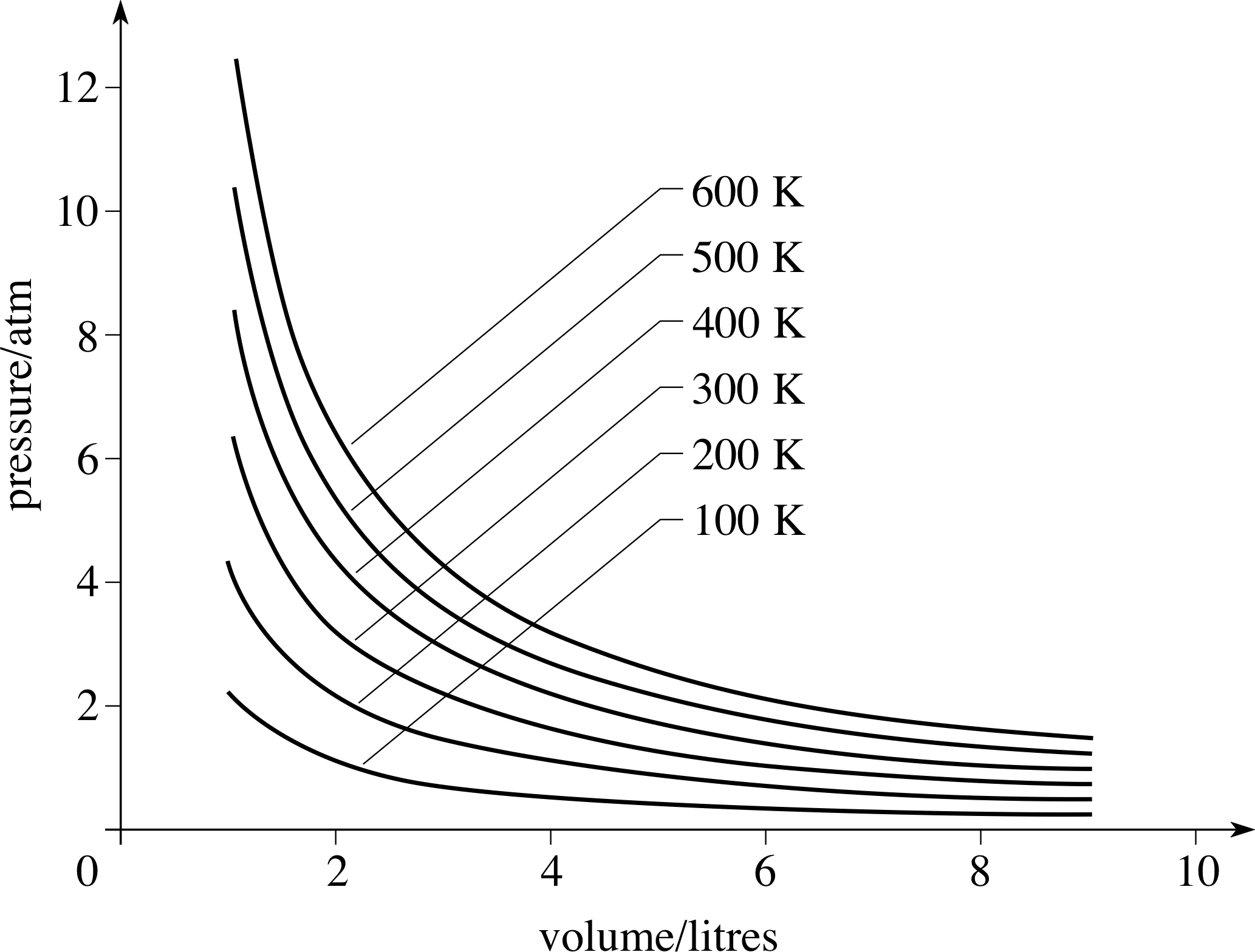
Figure 5 Isotherms for 1 g of helium, whose behaviour approximates very closely to that of an ideal gas.
The relationship described by Equation 29 may be shown on a graph of P against V, in fact such a curve was included in Figure 4a and several more such curves are shown in Figure 5. Curves of this general form are described geometrically as hyperbolae. Physically, any curve that represents an isothermal processes is called an isotherm. i
As Figure 5 indicates, for a fixed quantity of gas, the higher the temperature at which an isothermal process takes place, the higher the corresponding isotherm will be on the P−V graph.
In contrast to an isothermal process, an adiabatic process is one in which no heat passes in or out of the sample. If a gas expands adiabatically, its temperature falls: the gas does work at the expense of its own internal energy (∆W > 0, ∆U < 0, ∆Q = 0). If a gas is compressed adiabatically, its temperature rises: by pushing the plunger, you do work on the gas, i.e. you transfer energy to it (∆W < 0, ∆U > 0, ∆Q = 0). Note that in either case ∆Q = 0; this is the defining characteristic of any adiabatic process. i
For a fixed quantity of ideal gas undergoing a quasistatic process, it will always be the case that PV = nRT, but if the process is an adiabatic one the requirement that ∆Q = 0 will impose some further restriction on the relationship between P, V and T in any particular adiabatic process. What is this additional condition that distinguishes an adiabatic process from any other kind of process, i.e. what is the adiabatic counterpart of the isothermal condition of Equation 29? Let us find out!
Study comment The following discussion is quite detailed and ultimately requires some knowledge of calculus. If you have problems understanding the derivation consult your tutor about them when convenient, but for the moment go directly to the final result, Equation 37, and make sure you understand that.
Consider a process in which the pressure, volume and temperature of N moles of ideal gas change from P, V and T to P + ∆P, V + ∆V and T + ∆T, respectively. According to the first law of thermodynamics the heat that flows into the gas in such a process must be
∆Q = ∆U + ∆W(Eqn 4)
where ∆U is the change in the internal energy of the gas, which must be given by
∆U = nCV ∆T(Eqn 26) i
and ∆W is the work done by the gas.
If the pressure remained constant throughout the process we could write ∆W = P∆V, but P will not generally remain constant, so we can only use P∆V to determine the approximate value for the work done, and even then we must impose the additional requirement that the volume change ∆V should be small.
Hence∆Q ≈ nCV ∆T + P∆V(30)
where the approximation becomes increasingly accurate as ∆V is reduced.
Now suppose that the process described by Equation 30 is an adiabatic process, so that ∆Q = 0. Equation 30 then implies that in an adiabatic process
$\dfrac{-P\Delta V}{n\Delta T} \approx C_V$(31) i
We also know from the equation of state (PV = nRT) that at the end of the process (P + ∆P)(V + ∆V) = nR (T + ∆T)
i.e.PV + P∆V + V∆P ≈ nRT + nR∆T(32)
where the equation has become an approximation because we have neglected the term ∆P∆V on the grounds that it involves the product of two small quantities. Subtracting the right– and left–hand sides of the equation of state (PV = nRT) from the corresponding sides of Equation 32 we see that
P∆V + V∆P ≈ nR∆T(33)
i.e.$\dfrac{P\Delta V}{n\Delta T} + \dfrac{V\Delta P}{n\Delta T} \approx R$(34)
Using Equation 31 to eliminate P∆V/(n∆T) from Equation 34 we see that
$-C_V + \dfrac{V\Delta P}{n\Delta T} \approx R\quad\text{or}\quad C_V = \dfrac{V\Delta P}{n\Delta T} - R$
But we know from Equation 23,
CP − CV = R(Eqn 23)
so this last equation tells us that
$\dfrac{V\Delta P}{n\Delta T} \approx C_P$(35)
Dividing this expression for CP by that for CV above, and using Equation 33 to substitute for V∆P we see that
$\dfrac{-V\Delta P}{P\Delta V} \approx \dfrac{C_P}{C_V}$(36)
But CP /CV = γ, so we can rewrite Equation 36 as
$\dfrac{\Delta P}{\Delta V} \approx \dfrac{-p}{V}\gamma$
In the limit, as ∆V becomes vanishingly small, the left–hand side of this relation becomes the derivative dP/dV, and the approximation becomes an equality, so we obtain
$\dfrac{dP}{dV} = \dfrac{-\gamma P}{V}$
This is an example of a first–order differential equation, the solution of which (by the method of separation of variables) is fully described in the maths strand of FLAP (see the note below). The solution may be written in the form
PVγ = constant
Thus a fixed quantity of ideal gas undergoing an adiabatic process must satisfy
the adiabatic condition PVγ = constant(37)
Mathematical note The essential mathematical steps are:
Step 1 Treat dP and dV as though they are separate quantities and rewrite the differential equation as
$\dfrac{dP}{P} = -\gamma\dfrac{dV}{V}$
Step 2 Integrate both sides to obtain
$\displaystyle \int\dfrac{dP}{P} = \int\dfrac{-\gamma dV}{V}$
Step 3 Evaluate the integrals to obtain
$\loge\left(\dfrac{P}{P_0}\right) = -\gamma\loge\left(\dfrac{V}{V_0}\right) = \loge\left(\dfrac{V}{V_0}\right)^{-\gamma}$
where P0 and V0 are arbitrary constants with the dimensions of pressure and volume, respectively.
Step 4 Exponentiate both sides to obtain
P/P0 = (V/V0)−γ
i.e.PVγ = P0V0γ = constant
As in the case of the isothermal condition, the constant that appears in Equation 37 is characteristic of the adiabatic process being considered. Its value for any particular adiabatic process can be determined by the initial state of the process or from any other state the sample passes through during the process, so if (Pa, Va) and (Pb, Vb) are two such states, it follows from Equation 37 that
PaVaγ = PbVbγ
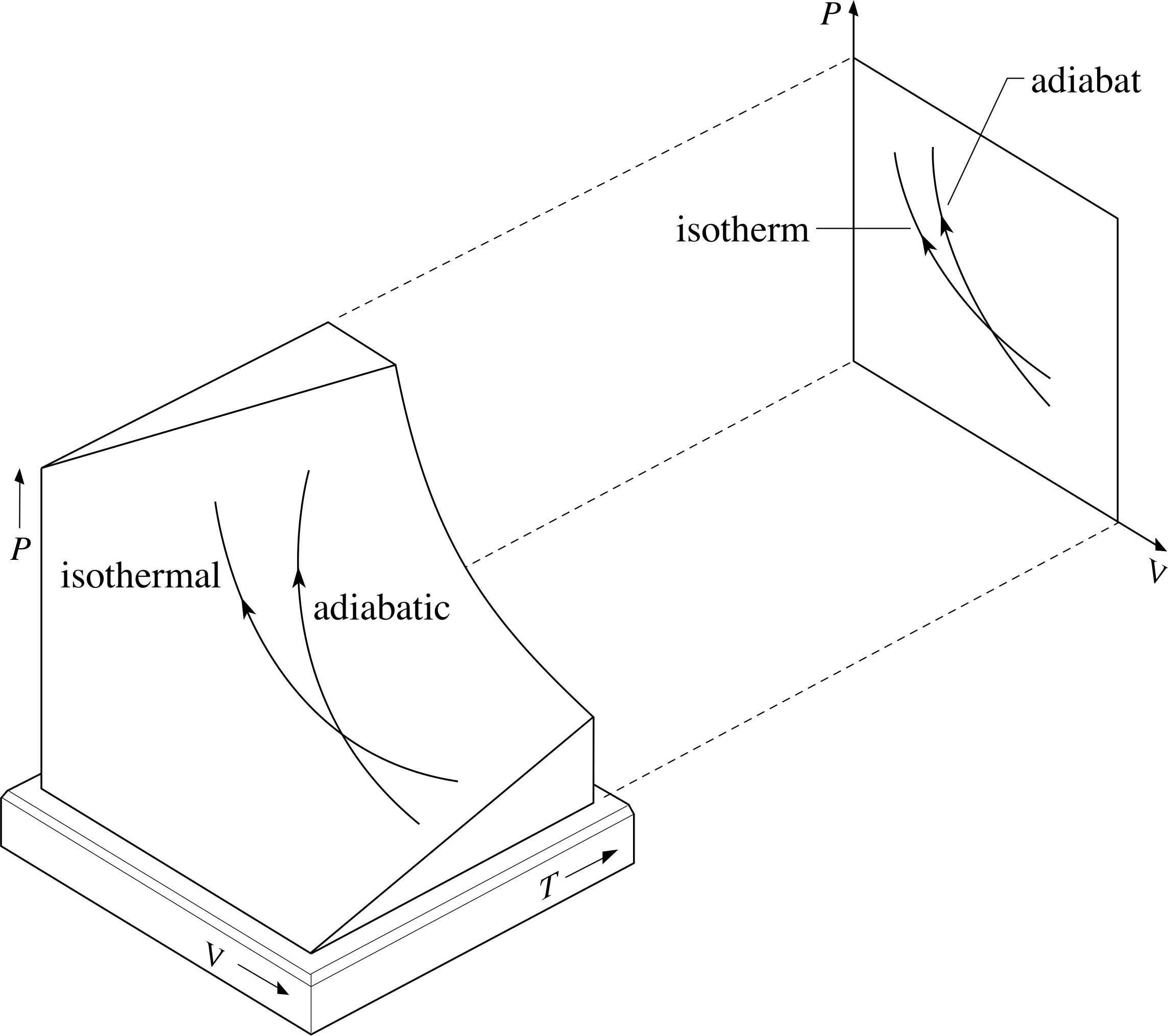
Figure 6 Adiabats and isotherms as projections from the PVT–surface of an ideal gas onto the P–V plane. At any point the adiabat is always steeper than the isotherm.
A curve representing an adiabatic process on a P–V graph is called an adiabat. Since γ is greater than 1 for all ideal gases it is always the case that an adiabat passing through any point will be steeper than an isotherm at the same point. Recalling that adiabats and isotherms are simply projections onto the P – V plane of what are really pathways on the PVT–surface makes it clear why this is so, as Figure 6 indicates.
Equation 37,
The adiabatic condition PVγ = constant(Eqn 37)
is the most commonly remembered equation describing reversible adiabatic changes in an ideal gas. i However, we can derive other equivalent expressions. From the equation of state (Equation 11),
PV = nRT(Eqn 11)
P = nRT/V, so $PV^\gamma = \dfrac{nRT}{V}V^\gamma = nRTV^{\gamma-1}$
Since nR is constant for a fixed quantity of gas we can say from Equation 37 that another condition that must be obeyed in an adiabatic process is
TV(γ −1) = constant(38) i
Notice that the constant referred to here will generally be different from that in Equation 37. We have not bothered to indicate that difference since its value will, in any case, differ from sample to sample and from process to process. It has a fixed value in each particular adiabatic process, but it is not a universal constant like R.
✦ Derive an equation relating T and P for an ideal gas undergoing an adiabatic change.
✧ From Equation 11,
PV = nRT(Eqn 11)
$V = \dfrac{nRT}{P}$, so $V^\gamma = \dfrac{(nR)^\gamma T^\gamma}{P^\gamma}$.
Hence,
$PV^\gamma = \dfrac{(nR)^\gamma T^\gamma P}{P^\gamma} =(nR)^\gamma T^\gamma P^{1-\gamma}$
It then follows from Equation 37,
PVγ = constant(Eqn 37)
that the adiabatic condition is,
TγP(1−γ) = constant
By raising this expression to the power 1/γ, we can write
TP(1−γ) = constant(39)
Question T12
Helium at 300 K and 1 atm pressure is compressed reversibly and adiabatically to a pressure of 5 atm. Assuming that helium under these conditions behaves as an ideal monatomic gas, what is the final temperature?
Answer T12
Using subscripts i and f to denote initial and final states, Equation 39,
TP(1−γ) = constant(Eqn 39)
gives TfPf(1/γ−1) = TiPi(1/γ−1), and so Tf = (Pi/Pf)(1/γ−1)Ti
Since the helium can be treated as a monatomic ideal gas, γ = 5/3. Hence, 1/γ = 3/5, and (1/γ1) − 1 = −2/5.
It follows that Tf = (1 atm/5 atm)−2/5 × 300 K = 52/5 × 300 K = 571 K.
Question T13
A fixed mass of gas is in an initial state A (P1, V1, T1). The gas expands adiabatically to a state B (P2, V2, T2). It is then heated at constant volume until it reaches the original temperature, i.e. state C has (P3, V2, T1).
(a) On a P−V graph, sketch the isotherms for temperatures T1 and T2.
(b) On the same graph draw the path from state A, via state B, to state C.
(c) If T1 = 300 K, V2 = 4V1, and γ = 7/5 what is T2?
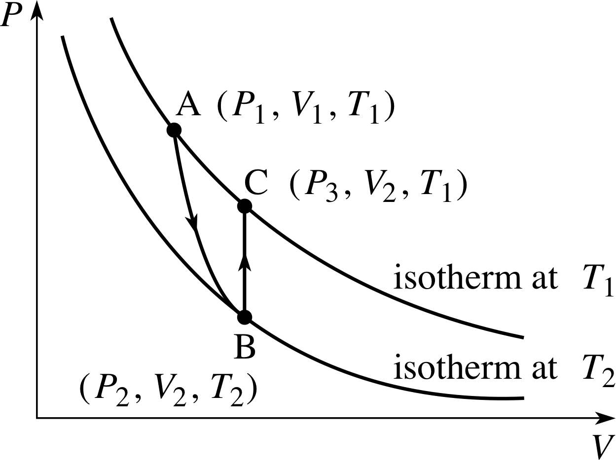
Figure 19 See Answer T13.
Answer T13
(a) The P–V graph is given in Figure 19.
(b) The path is given in Figure 19.
(c) From Equation 38,
TV(γ −1) = constant(Eqn 38)
T1V1γ−1 = T2V2γ−1 = constant
So,T2 = T1(V1/V2)(γ−1) = (1/4)0.4 × 300 K = 172 K
4 PVT–surfaces and changes of phase
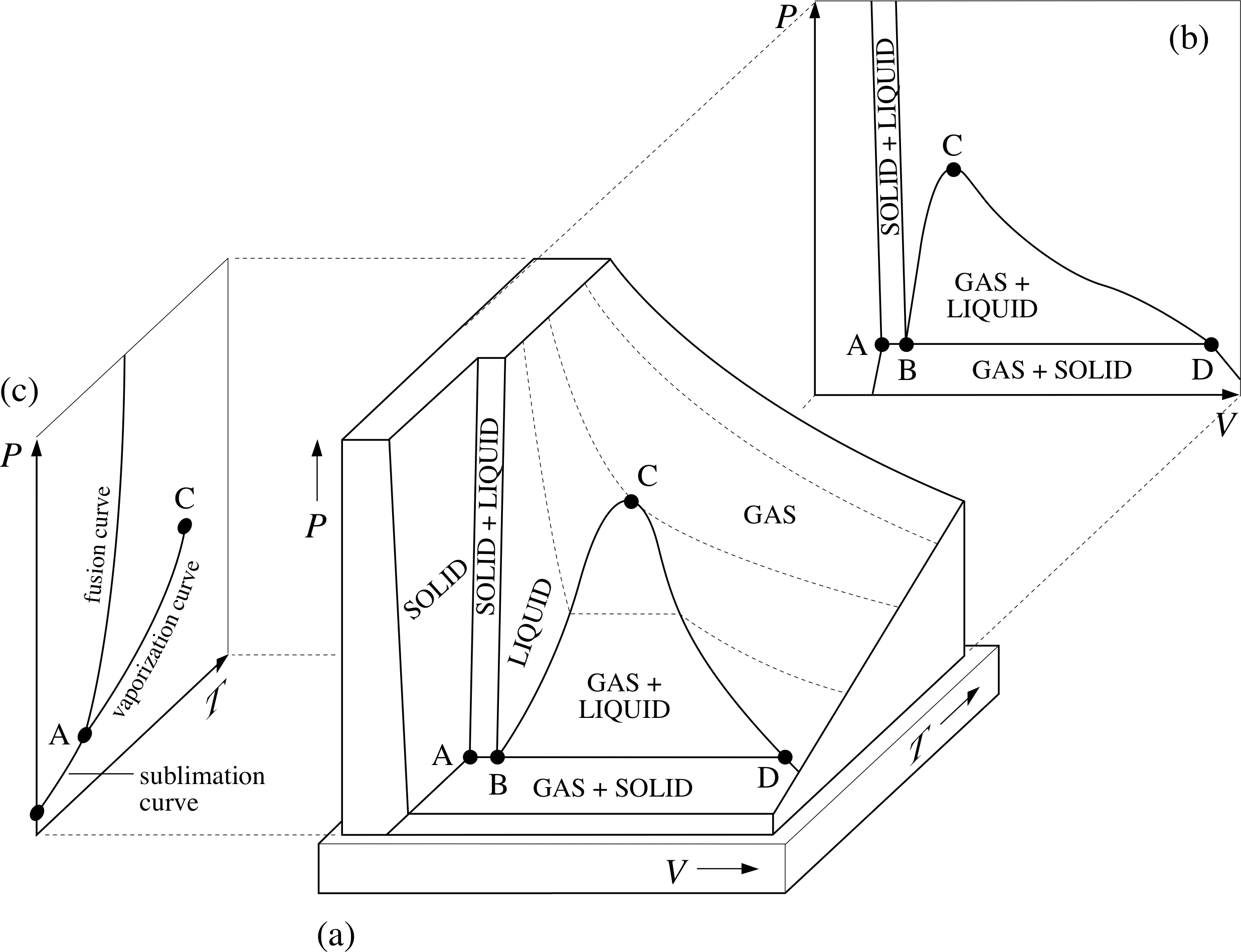
Figure 7 (a) The generic PVT–surface for a fixed quantity of a typical substance. The dotted lines show paths of constant temperature on the PVT–surface. (b) The projection of the PVT-surface onto the P–V plane. (c) The projection of the PVT–surface onto the P–T plane.
Figure 7a shows the PVT–surface for a fixed quantity of a typical substance, sometimes called the generic PVT–surface.
The surface has been truncated for ease of display, but in principle it includes all the equilibrium states of the given sample. As was the case with the corresponding UPT surface (Figure 1), it includes regions that correspond to the liquid and solid phases, as well as the gas phase, and there are also regions in which different phases coexist.
These regions of coexistence can be clearly seen when the generic PVT-surface is projected onto the P–V plane (Figure 7b), but a projection onto the P–T plane merely shows them as boundaries between the single phase regions (Figure 7c). As stated earlier, a quasistatic process corresponds to a pathway on the PVT–surface; if the projection of such a pathway onto the P–T plane crosses one of the boundaries between different phases then that process will involve a phase transition such as fusion, vaporization or sublimation.
For that reason the boundaries seen on the P–T plane are called the fusion curve, the vaporization curve and the sublimation curve. The purpose of this section is to introduce you to some of the special features of the generic PVT–surface and its projections as they relate to phase transitions and the latent heats that accompany them. i
4.1 The critical point
As Figure 7a indicates, at high temperature and moderate pressure the typical substance is a gas, with isotherms on the P–V plane that look pretty much like the hyperbolae that characterize an ideal gas. At somewhat lower temperatures the behaviour is rather different; below a certain temperature, T c, corresponding to the constant temperature pathway through the point marked C in Figure 7, isotherms pass through the region corresponding to the liquid phase as well as the gas phase.
| Substance (1 mol) | Pc/105 Pa | Vc/10−6 m3 | Tc/ K |
|---|---|---|---|
| argon (Ar) | 49 | 75 | 151 |
| nitrogen (N2) | 34 | 89 | 126 |
| carbon dioxide (CO2) | 74 | 94 | 304 |
| water (H2O) | 221 | 56 | 647 |
| hydrogen (H2) | 13 | 65 | 33 |
These subcritical (T < Tc) isotherms also include a flat segment, corresponding to their passage across the region in which gas and liquid coexist. The point C that marks the high temperature limit to gas/liquid coexistence is obviously of particular interest. It is called the critical point and the values of temperature pressure and volume that determine its location for a given sample are called the critical temperature, Tc, the critical pressure, Pc, and the critical volume, Vc, for that sample.
Critical point data for one mole samples of various substances are listed in Table 2.
As you can see from the P–T plane in Figure 7c, the critical point C marks the end of the vaporization curve. This means that the distinction between the gas phase and the liquid phase ceases to be very clear in the neighbourhood of the critical point. A gas is so dense under near–critical conditions that it is essentially indistinguishable from a liquid at that point.
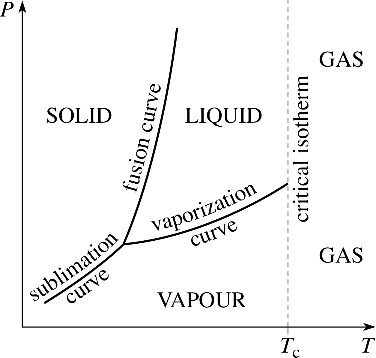
Figure 8 Using the critical isotherm to arbitrarily distinguish a liquid and a vapour from a gas.
Indeed, the fact that the vaporization curve ends at the critical point means that it is always possible to find a process whereby a gas can be converted into a liquid by a combination of heating compression and cooling, without undergoing a phase transition at all. This inevitably means that the distinction between a liquid and a dense gas is somewhat arbitrary. One common way of distinguishing liquids from dense gases despite the absence of any real difference between them is to accept the critical isotherm (T = Tc) as an arbitrary dividing line. The region of the P–T plane between the fusion curve, the vaporization curve and the critical isotherm then unambiguously belongs to the liquid phase. In a similar spirit a gas below the critical temperature is sometimes referred to as a vapour. This naming convention is indicated in Figure 8. i
Using this terminology we can say that the vaporization curve of a sample represents the range of conditions under which a liquid and its vapour can coexist in equilibrium. A vapour that is in this state of coexistence is said to be a saturated vapour, and, as the P–T graph shows, its pressure will be a function of temperature only for a given substance.
The vaporization curve of a substance may therefore be said to show the variation of the saturated vapour pressure with temperature. Any attempt to quasistatically compress or expand a saturated vapour, without changing its temperature, simply results in more of the vapour condensing, or more of the liquid evaporating.

Figure 7a The generic PVT–surface for a fixed quantity of a typical substance. The dotted lines show paths of constant temperature on the PVT–surface.
Question T14
(a) Using a pencil, mark two points on Figure 7a, one clearly belonging to the liquid phase, the other clearly corresponding to an unsaturated vapour.
(b) Draw two separate paths on the PVT–surface, representing quasistatic processes whereby one of the states you marked might be reached from the other, with one process involving only a single phase transition and the other involving no phase transition at all.
(c) Sketch the projections of your two pathways onto the P–V and P–T planes. (Once you have answered this question it might be a good idea to erase your pencil marks from Figure 7 to avoid future confusion.)
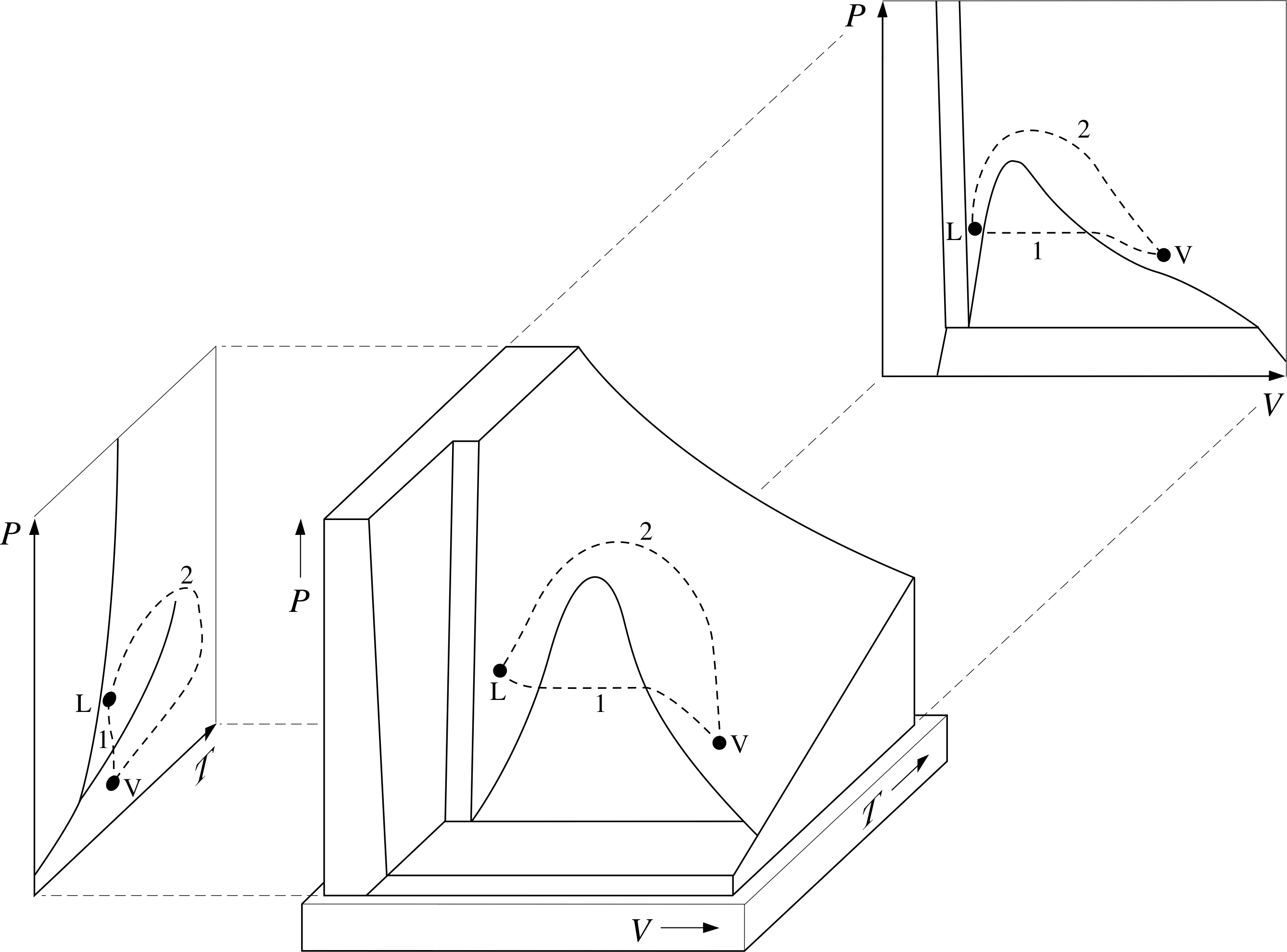
Figure 20 See Answer T14.
Answer T14
(a) The point L on Figure 20 represents a state in the liquid phase, and V a state in the vapour phase.
(b) Path 1 represents a process involving a single phase transition, path 2 involves no phase transition as such even though the phase is changed.
(c) The projections on the P–V and P–T surfaces are also shown in Figure 20.
It is interesting to consider just what happens to a sample when it undergoes a process that takes it near its critical point, and to compare that behaviour with processes that do not involve the critical point. As an example of the latter consider heating an equilibrium mixture of liquid and vapour in a transparent container of fixed volume. The initial state of such a mixture will be represented by a point on the liquid/gas coexistence region and the heating will cause the state to move along a path parallel to the T-axis, in the direction of increasing temperature.
If the sample has a critical volume that is less than the volume of the container (Vc < V) the heating will not cause the sample to pass through its critical point. All that happens is that the temperature and pressure rise while the proportion of liquid decreases. During this process, the surface that separates the gas from the liquid (the meniscus) falls until it disappears when all the liquid has vaporized and the container is entirely full of gas. The meniscus is clearly visible when there is some liquid and it is absent when there is not – a very straightforward situation.
If you repeat the process, but start with an equilibrium mixture of liquid and vapour that has a critical volume greater than the volume of the container (Vc > V), the outcome is rather different. Heating at constant volume will again cause the temperature and pressure to rise, but this time the proportion of liquid in the container will increase, the meniscus will rise and the sample will become entirely liquid once all the gas has condensed. Despite this difference, the disappearance of the gas is easy to see if one keeps one’s eye on the meniscus.
Now, compare the above descriptions with what happens when the critical volume of the sample exactly equals the volume of the container. This time raising the temperature while holding the volume constant will cause the mixture of liquid and vapour to approach its critical point. The outcome is curious and quite striking to observe.
As the critical point is approached, the usually clear meniscus between the liquid and the gas becomes more indistinct until at T = Tc we cannot tell one phase from the other. The sample becomes cloudy (with so–called critical opalescence), and careful measurements of a number of properties including specific heat, compressibility, and thermal conductivity reveal anomalies which have only been properly understood in the last 25 years.
4.2 The triple point
Figure 7a The generic PVT–surface for a fixed quantity of a typical substance. The dotted lines show paths of constant temperature on the PVT–surface.
The horizontal line ABD in Figure 7a marks the meeting place of the various regions in which pairs of different phases coexist; as a result, all three phases of matter can coexist along ABD which is accordingly called the triple–point line.
For a given sample, the triple–point line covers a range of volumes, but it always occurs at unique values of pressure and temperature. Its projection onto the P–T plane therefore consists of a single point, called the triple point (point A in Figure 7). As explained elsewhere in FLAP the triple–point temperature of H2O (defined as 273.16 K = 0.00 °C) is so accurately reproducible that it is used as one of the fundamental calibration temperatures in modern thermometry.
| Substance (1 mol) | Ptr/105 Pa | Vtr/10−6 m3 | Ttr/K |
|---|---|---|---|
| argon (Ar) | 0.68 | 28 | 84 |
| nitrogen (N2) | 0.12 | 17 | 63 |
| carbon dioxide (CO2) | 5.10 | 42 | 216 |
| water (H2O) | 0.006 | 18 | 273.16 |
| hydrogen (H2) | 0.072 | 25 | 14 |
| The triple point volumes quoted are for the liquid phase. There are different values for the solid and gas phases. |
|||
Some data concerning triple–point pressure, triple–point temperature and triple–point volume for one mole samples of various substances are given in Table 3.
✦ For a given sample, how do P, V and T change from one end of the triple–point line to the other?
✧ Since the line runs parallel to the V–axis, neither P nor T changes. The triple–point line is both an isobar (a line of constant pressure) and an isotherm.
One end of the triple–point line corresponds to a relatively large volume and represents a state in which the sample is entirely vapour (i.e. gas).
The other end of the line corresponds to a smaller volume and represents a state in which the sample is entirely solid.
Intermediate points along the line correspond to intermediate volumes and states in which different proportions of gas, liquid and solid coexist.
The triple–point line on a PVT–surface may be visualized as being like a horizontal ridge on a mountain, where two distinct ski–slopes from higher up the mountain combine to form one which leads down to the foothills. There are three different ski–slope gradients but the edge of the ridge is strictly a straight line. You can model the geometry by folding a piece of cardboard like a greetings card, then making a cut on one side running down perpendicularly to the fold, cutting shapes corresponding to the solid-plus-liquid and liquid-plus-vapour phase mixtures, and finally adjusting the angles of the three planes relative to the fold so as to imitate the shapes shown in Figure 7.
If you look along the fold you see it as a point: when it is represented as a two–dimensional P–T projection such as the one shown in Figure 7c, it is the point where areas representing solid, liquid and vapour phases converge.
Throughout this section we have based all of our discussions on the generic PVT–surface of Figure 7, but it is important to realise that many forms of matter show exceptional behaviour of one kind or another. A good case in point is H2O which can exist as ice, water or steam. H2O is a common material, but its behaviour is not simple.
Compare its PVT–surface, as shown in Figure 9, with the generic surface of Figure 7. Notice the odd behaviour to the left of the triple–point line for H2O: the ice-and-water surface slopes ‘the wrong way’. This is because water expands when it freezes, whereas more typical substances contract when they freeze. This quirk in the behaviour of water enables ice to float on water and thereby permits aquatic pond life to survive freezing conditions that might otherwise be lethal.
In addition to the familiar liquid and vapour phases, H2O also has a whole portfolio of high pressure solid phases, which all have different crystal structures and densities. Figure 10 shows some of these phases. Note that Figure 9 represents a small part of this larger scale surface.
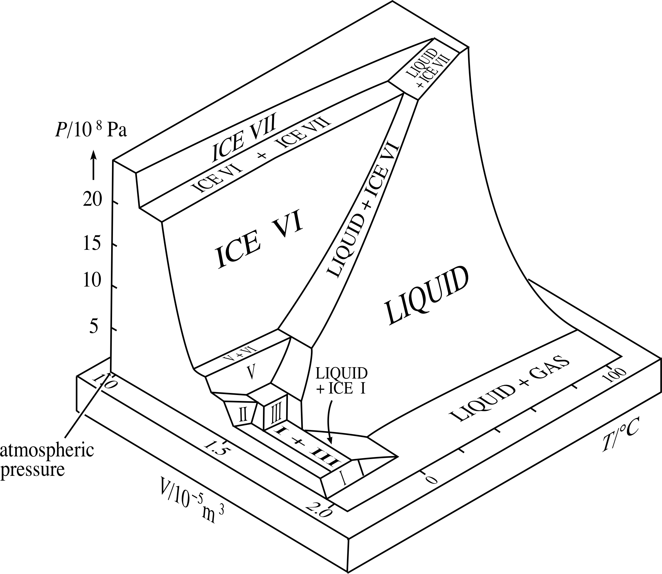
Figure 10 Part of the PVT–surface for H2O. Note that the range of pressures is much greater than in Figure 9.
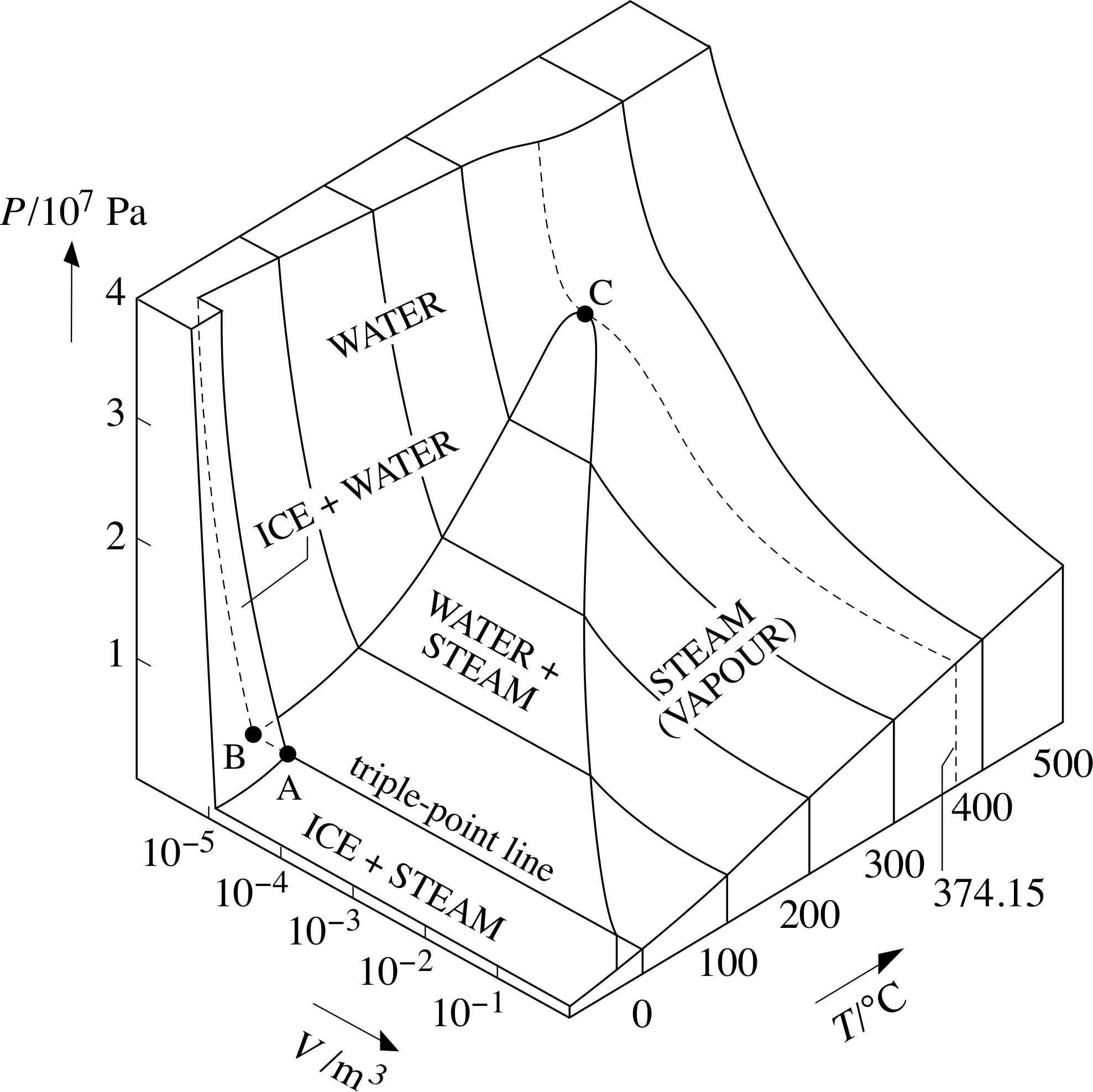
Figure 9 A PVT–surface for H2O. (For a sample containing 1 mole.)
4.3 The Clausius–Clapeyron equation
An isothermal process that crosses any of the boundary curves seen in the P–T plane – the vaporization curve, the fusion curve, or the sublimation curve – involves the absorption or emission of latent heat, while a change of volume takes place. The volume change cannot be seen from the P–T graph, but it can be gauged from the corresponding P–V graph or from the PVT–surface itself. The Clausius–Clapeyron equation provides an interesting and useful link between the slope of the interphase boundary at any relevant point in the P–T plane and the latent heat ml and volume change ∆V involved in crossing it. i The equation may be written in the form
Clausius–Clapeyron equation $\dfrac{dP}{dT} = \dfrac{ml}{T\Delta V}$(40)
where m is the mass of the sample, l the relevant specific latent heat absorbed by the sample, ∆V the increase in volume of the sample and T the absolute temperature at which the process takes place. Note that in the case of ice, where melting involves a decrease in volume (and hence a negative ∆V) but an absorption of latent heat (and hence a positive l) the Clausius–Clapeyron equation predicts a negative value for the gradient of the fusion curve, in agreement with the behaviour shown in Figure 9. The Clausius–Clapeyron equation is considered in the maths strand of FLAP, where it is shown that if ml = nL is treated as a constant, and if we suppose ∆V = nRT/P (which is equivalent to assuming that we are dealing with the process of vaporization and treating the volume of the liquid as negligible compared with the volume of the vapour, which is itself treated as an ideal gas) then the saturated vapour pressure is related to the temperature by the expression
P = C e−L/RT
In view of the crudity of the assumptions, this expression provides a surprisingly good description of the vaporization curve of various substances.
5 Entropy and the second law of thermodynamics
We end this module with a discussion of the second law of thermodynamics which will lead us to introduce a function of state called entropy. The entropy of a sample is in some ways comparable to the sample’s internal energy; that too is a function of state introduced in response to a law of thermodynamics (the first law in that case). However, as you will see there are also very great differences between entropy and internal energy.
In what follows it will be useful to make an especially clear distinction between the object or sample being studied, which we will call the system, and the rest of the universe, which we will call the environment. Throughout most of this module we have been concerned with the effect on a system (e.g. a fixed quantity of ideal gas) of transferring a given quantity of energy to it or from it. In the rest of the module we must remember that the energy transferred to or from a system can only come from or go to its environment.
With the environment in mind we can also introduce another important distinction, that between a reversible and an irreversible process. Almost any process can be reversed in the sense that whatever changes are made to a system can be undone; a compressed gas can be allowed to expand, a broken plate can be repaired. However a process is only reversible in the technical sense if both the system and its environment can be returned to their original states after the process has taken place. As you will see this is often not possible; processes that involve friction, viscosity or other dissipative effects will always turn out to be irreversible_processirreversible when analysed with sufficient care.
You might be able to repair a broken plate and literally make it as good as new, but in doing so you will irreversibly change the environment, so the process of breaking a plate is technically irreversible, despite the possibility of repairing the plate itself. In practice almost every real process is irreversible: that is why we have such a clear sense of the direction of time. The second law of thermodynamics and the concept of entropy help us understand the irreversibility of nature and thereby provide a starting point for discussions of the origin of the physical distinction between past and future, the ‘arrow of time’ as it is known in physics.
5.1 The second law of thermodynamics
Two objects in thermal contact, initially at the same temperature, never display a spontaneously widening temperature difference, nor does a hot object in contact with a cold object spontaneously increase its temperature by transferring energy from the colder object. Why not? Neither of these processes would violate the energy conservation expressed in the first law of thermodynamics. The first law of thermodynamics does not, therefore, tell us the complete story about processes involving heat and work. It forbids certain processes from happening, but it does not tell us which energy conserving processes will happen spontaneously. We can formalize our observations about spontaneously occurring processes by stating:
the second_law_of_thermodynamicssecond law of thermodynamics (Clausius form):
No process is possible whose sole result is the transfer of heat from a colder to a hotter body.
Note the crucial term ‘sole result’ in this law; it is certainly possible to transfer heat from a colder to a hotter body, refrigerators do that all the time, but it is certainly not their sole result; they only achieve it by consuming electricity or gas and transferring more heat to their environment than they transfer from their interior. (Leaving a fridge door open is a way of warming a room!)
The Clausius form of the second law of thermodynamics may seem an innocuous statement of everyday experience, but its implications are far reaching. The first thing to note is that it can be stated in the following equivalent form:
the second_law_of_thermodynamicssecond law of thermodynamics (Kelvin form):
No process is possible whose sole result is to transfer a given quantity of heat from a body and convert it entirely into work. i
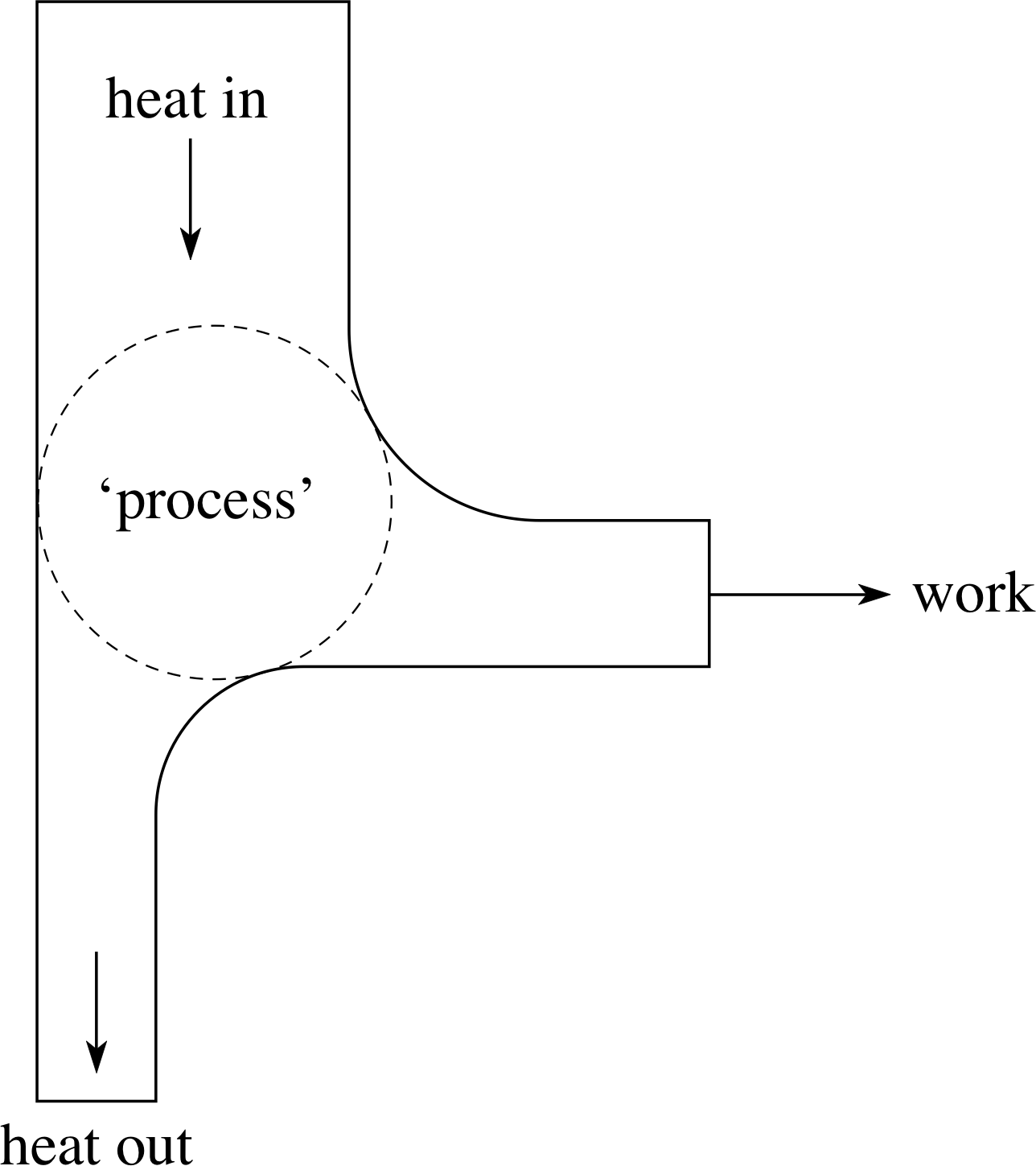
Figure 11 A schematic representation of the second law of thermodynamics (Kelvin form).
Again, it is important to note the term ‘sole result’ in this law. Internal combustion engines convert the heat transferred from a burning mixture of air and petrol into work, but that is not their sole result; they also produce exhaust gases and warm their environment. The Kelvin form of the second law also makes it clear that the conversion of heat to work must always be an incomplete process; since all methods of transferring energy can be classified as either heat or work the impossibility of completely converting a given quantity of heat into work means that some heat must always be ‘left over’ in a conversion process that has no other effect. This is indicated schematically in Figure 11.
The equivalence of the Clausius and Kelvin forms of the second law can be proved by showing that the violation of either statement implies the violation of the other. For example, suppose you knew of a process that violated the Kelvin form of the second law, then you could use that process to transfer a quantity of heat ∆Q from a body at temperature T1 and convert it entirely into an equivalent amount of work ∆W, without any other effect. You could then use all that work, possibly in the form of frictional rubbing or stirring, to raise the temperature of some other body initially at temperature T2.
When this two step process was complete its overall effect would be equivalent to transferring a quantity of heat ∆Q from the body at temperature T1 to the body at temperature T2. However, there was nothing in the argument to prevent T2 from being greater than T1, so you could use your Kelvin violating process to transfer heat from a colder to a hotter body, thereby violating the Clausius form. A similar argument shows that a violation of the Clausius form implies a violation of the Kelvin form, so the two forms are indeed equivalent.
Figure 12 Energy flow in a heat engine.
Now in order to grasp the implications of the Kelvin form of the second law it is useful to introduce the idea of a heat engine. This is a device (shown schematically in Figure 12) that transfers energy, in the form of heat Q1, from part of the environment at constant temperature T1, converts part of that energy into work ∆W and transfers the remainder, in the form of heat Q2, back into part of the environment at constant temperature T2. i
The constant temperature parts of the environment are generally referred to as thermal reservoirs, implying that heat may be transferred to or from them without altering their temperature or causing any irreversible disturbance. The conversion of heat into work
is carried out within the engine by a thermodynamic system that works in a closed cycle, by which we mean that the system returns to its original state at the end of each cycle. The construction of such an engine is of course consistent with the first and second laws of thermodynamics. A real steam engine that lets hot steam enter a cylinder (thereby transferring heat from the environment), allows the steam to expand almost adiabatically (thereby doing work while cooling the steam), vents the cooled steam (thereby transferring heat to the environment) and then returns the cylinder to its original volume, ready for the next influx of steam, provides a good model of a heat engine.
Note Many of the ideas of thermodynamics were developed in the mid 19th century when there was great interest in improving the efficiency of industrial steam engines. Don’t get the idea that steam engines are old–fashioned – they drive the turbines in our most modern power stations.
Since a heat engine returns to its original state after each cycle, it follows that the net change in its internal energy over a complete cycle is ∆U = 0. The first law of thermodynamics (∆Q = ∆U + ∆W) with ∆U = 0 therefore tells us that over a complete cycle
Q1 − Q2 = ∆W(41)
The efficiency η of a machine is the ratio of the useful work it performs to the energy it consumes. If we assume that none of the work performed by the heat engine is wasted due to friction or any other dissipative effect we can say that its efficiency will be
$\eta = \dfrac{\Delta W}{Q_1} = \dfrac{Q_1-Q_2}{Q_1} = 1 -\dfrac{Q_2}{Q_1}$(42a) i
Now in the absence of friction and other dissipative effects, a heat engine will be reversible. That is to say if heat Q2 is transferred to the engine from a thermal reservoir at temperature T2, and if the environment does work ∆W on the heat engine, then heat Q1 can be transferred from the engine to a reservoir at temperature T1, thereby returning both the system and its environment to their original states, and satisfying the requirement for reversibility that was stated earlier. i
Since the expression on the right–hand side of Equation 42a applies to a reversible heat engine we will henceforth refer to it as the efficiency of a reversible heat engine and write
$\eta_{\rm rev} = 1-\dfrac{Q_2}{Q_1}$(42b)
Figure 13 (a) A Carnot cycle consisting of two isothermal processes and two adiabatic processes. Four of the states involved in the process are marked A, B, C, D. (b) The Carnot engine procedures that correspond to the four steps of a Carnot cycle. Steps A → B and C → D are slow, steps B → C and D → A are fast.
If we want to work out the efficiency of a particular reversible heat engine we obviously need to know the values of Q2 and Q1. One particular kind of reversible heat engine for which this is possible is the so–called Carnot engine, which uses a cyclic process called the Carnot cycle. i A Carnot cycle consists of four steps; two of them are isothermal processes at temperatures T1 and T2, during which quantities of heat Q1 and Q2 are transferred to and from the system, and the other two steps are adiabatic processes that bring about the temperature changes needed to link one isothermal process to the other. The whole cycle is shown in Figure 13a.
The corresponding operations of a Carnot engine – in this case a cylinder fitted with a piston and filled with ideal gas – are shown in Figure 13b. Starting with the Carnot engine in thermal equilibrium with a thermal reservoir at temperature T 2 (corresponding to state A in Figure 13a) the Carnot cycle involves the following operations.
- A → B
-
Quasistatically and reversibly compress the gas while maintaining equilibrium with the reservoir at temperature T2. This will be an isothermal process that will increase the pressure of the gas. i Because ∆T = 0, and the gas is ideal it follows that ∆U = 0. The first law of thermodynamics then implies that the heat supplied to the gas ∆Q = ∆W, where ∆W is the work done by the gas. In this case ∆Q = −Q2, and it can be shown that ∆W = nRT2 loge(VB/VA). It follows that Q2 = 1 − nRT2 loge(VB/VA). This will be a positive quantity since VB/VA < 1.
- B → C
-
Thermally isolate the gas, and compress it quasistatically and reversibly until its temperature is T1. This will be an adiabatic process that will further increase the pressure of the gas. Because ∆Q = 0, the first law of thermodynamics implies that ∆U = −∆W. In this case ∆U will be positive since the temperature of the gas increases.
- C → D
-
Allow the gas to expand quasistatically and reversibly while maintaining equilibrium with the reservoir at temperature T1. This will be an isothermal process that will decrease the pressure of the gas. Because ∆T = 0, and the gas is ideal, it follows that ∆U = 0. The first law of thermodynamics then implies that the heat supplied to the gas ∆Q = ∆W, where ∆W is PB the work done by the gas. In this case ∆Q = Q1, and it can be shown that ∆W = nRT1 loge(VD/VC.). It follows that Q1 = nRT1 loge(VD/VC). Note that this will be a positive quantity because VD/VC > 1.
- D → A
-
Thermally isolate the gas, and allow it to expand quasistatically and reversibly until its temperature is again T2. This will be an adiabatic process that will return the system to its original state. Because ∆Q = 0, the first law of thermodynamics implies that ∆U = −∆W. In this case ∆U will be negative since the temperature of the gas decreases.
It follows from the values for Q1 and Q2 given above that in this case the efficiency of the reversible engine will be
$\eta_{\rm rev}= 1 - \dfrac{Q_2}{Q_1} = 1- \left[\dfrac{-nRT_2\loge(V_{\rm B}/V_{\rm A})}{nRT_1\loge(V_{\rm D}/V_{\rm C})}\right]$
Question T15
Use the adiabatic condition in the form TV(γ−1) = constant, derived in Subsection 3.4, to obtain an expression for loge(VB/VA)/loge(VD/VC) and hence show that in a Carnot cycle:
$\dfrac{Q_1}{T_1} = \dfrac{Q_2}{T_2}$(43) i
Figure 13 (a) A Carnot cycle consisting of two isothermal processes and two adiabatic processes. Four of the states involved in the process are marked A, B, C, D. (b) The Carnot engine procedures that correspond to the four steps of a Carnot cycle. Steps A → B and C → D are slow, steps B → C and D → A are fast.
Answer T15
Applying the adiabatic condition to the process that leads from B to C:
T2VB(γ−1) = T1VC(γ−1)
Applying the adiabatic B condition to the process that leads from D to A:
T1VD(γ−1) = T2VA(γ−1)
Dividing the right–hand side of the first equation by the left–hand side of the second and vice versa we see that:
$\dfrac{V_{\rm B}^{(\gamma-1)}}{V_{\rm A}^{(\gamma-1)}} = \dfrac{V_{\rm C}^{(\gamma-1)}}{V_{\rm D}^{(\gamma-1)}}$
which implies that
$\dfrac{V_{\rm B}}{V_{\rm A}} = \dfrac{V_{\rm C}}{V_{\rm D}}$
hence
$\dfrac{\loge(V_{\rm B}/V_{\rm A})}{\loge(V_{\rm D}/V_{\rm C})} = \dfrac{\loge(V_{\rm B}/V_{\rm A})}{\loge(V_{\rm C}/V_{\rm D})^{-1}} = -1$
It follows that $\dfrac{Q_2}{Q_1} = \left(\dfrac{-nRT_2\loge(V_{\rm B}/V_{\rm A})}{nRT_1\loge(V_{\rm D}/V_{\rm C})}\right) = \dfrac{T_2}{T_1}$
so, as required, $\dfrac{Q_1}{T_1} = \dfrac{Q_2}{T_2}$(Eqn 43)
This relation is important in its own right and we will consider its general implications very shortly. For the moment, however, we will just use it to rewrite the expression for the efficiency of a Carnot engine
$\eta_{\rm rev} = 1 -\dfrac{T_2}{T_1}$(44) i
As you can see, the efficiency of the reversible Carnot engine we have been considering is entirely determined by the absolute temperatures between which it operates. The smaller the value of T2/T1 the more efficient the engine. But the engine cannot be totally efficient unless T2 = 0 K, and attaining absolute zero is impossible both in practice and in principle. i
The result we have just derived is pleasingly simple, but if it were limited to a Carnot engine filled with ideal gas it would hardly have been worth the effort we have put into deriving it. Fortunately that is not the case due to the following results which we state without proof:
- 1
-
No heat engine operating between two fixed temperatures can have greater efficiency than a reversible heat engine operating between those same two temperatures.
- 2
-
All reversible heat engines operating between two thermal reservoirs at fixed temperatures have the same efficiency.
It follows from these results that although we obtained Equation 44 by considering a Carnot engine filled with ideal gas, the result holds true for any reversible heat engine, irrespective of the system it contains. (The same may also be shown to be true of Equation 43). Furthermore, no other heat engine could be more efficient, so Equation 44 represents the efficiency of the ideal reversible heat engine. It thus gives a quantitative insight into the extent to which heat can be converted into useful work.
Question T16
Compare the efficiency of a modern steam generating plant operating between temperatures of 650 °C and 40 °C with that of an early steam engine operating between 120 °C and 80 °C. Why, in practice, would the efficiency of each engine be less than the values you have calculated?
Answer T16
Modern engine: T1 = 650 °C = 923 K, T2 = 40 °C = 313 K, so from Equation 44,
$\eta_{\rm rev} = 1 - \dfrac{T_2}{T_1}$(Eqn 44)
efficiency = 1 − (313/923) = 0.66 (often expressed as 66%).
Early engine: T1 = 393 K, T2 = 353 K, so efficiency = 1 − (353/393) = 0.10 (i.e. 10%).
In practice, there will be irreversible processes (e.g. due to friction in moving parts) so the useful work will be a smaller fraction of the energy input, and the true efficiencies less than these ideal values. (Even in a modern engine, the maximum practical efficiency is about 40%.)
5.2 Entropy: a function of state
The second law of thermodynamics points out the impossibility of completely converting a given amount of heat into work without any other effect. The discussion of reversible heat engines puts a quantitative limit on that conversion. From Equation 43 we can say that in the case of a reversible heat engine operating between fixed temperatures T1 and T2 the amount of heat that cannot be converted into work, Q2, must be sufficiently great that
$\dfrac{Q_1}{T_1} = \dfrac{Q_2}{T_2}$(Eqn 43)
This view suggests that the quantities Q1/T1 and Q2/T2 might have some special significance in the context of reversible energy conversions. This is indeed the case, as Clausius was the first to recognize. In fact Q1/T1 and Q2/T2 represent equal amounts of a quantity Clausius named entropy being transferred to and from the system. i Entropy, unlike energy, is not generally conserved. However, it does happen to be conserved in reversible processes; that is what distinguishes reversible processes from irreversible ones.
Figure 1 The variation with temperature and pressure of the internal energy U of a fixed quantity of a typical substance. Note that there are vertical regions on the UPT surface (corresponding to changes of phase) in which a change in internal energy is not necessarily accompanied by a change in temperature.
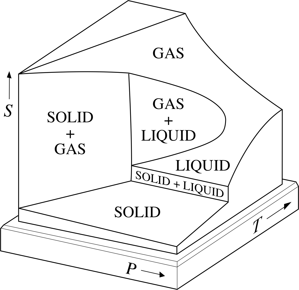
Figure 14 The SPT–surface for a fixed quantity of a given substance. This may be compared with the UPT surface of Figure 1.
The entropy S of a system is a function of state, like the internal energy. Like the internal energy, the entropy of a given system involves an arbitrary constant, but once a value has been assigned to this the entropy of every state has a unique value. i A highly schematic SPT–surface for a fixed quantity of a typical substance is shown in Figure 14. This is comparable to the UPT–surface of Figure 1.
Even without assigning a value to the arbitrary constant is still possible to discuss the difference in entropy between any two states of a system, since it is these differences in entropy that are physically significant and the arbitrary constant will not affect them.
What is the difference in entropy between any two given states? This question has a straightforward general answer, but it is a little complicated, so let us first consider a special case in which the answer is particularly simple. Suppose we have two equilibrium states, a and b, and that state b can be reached from state a by an isothermal process in which a quantity of heat ∆Qrev is reversibly transferred to the system at fixed temperature T. The difference in entropy between the two states, ∆S = Sb − Sa will then be given by
$\Delta S = \dfrac{\Delta Q_{\rm rev}}{T}$ (isothermal case)(45)
Note that we have specified that the heat must be transferred reversibly. This is necessary because heat is not a function of state and the heat transfer involved in a process will depend on the details of that process. By specifying that the process should be reversible, (as well as quasistatic and isothermal) we ensure that the heat transfer is uniquely specified.
In the general case it may not be possible to find an isothermal process linking two given states, and Equation cannot then be applied because there will be no unique value of T associated with any reversible process that leads from one state to the other. Under such circumstances we may find an approximate value for the entropy difference by identifying any convenient reversible process from one state to the other; dividing it into n small steps each involving the reversible transfer of heat ∆Qi at an approximately constant temperature Ti; and then adding together all of those small contributions. Thus:
$\displaystyle \Delta S \approx \sum_{i=1}^n\left(\dfrac{\Delta Q_i}{T_i}\right)$
This approximation will become more accurate as the increments ∆Qi are made smaller and their number correspondingly increased. In the limit as the largest ∆Qi becomes vanishingly small the approximation becomes an equality and we write the limit of the sum as a line integral i giving:
$\displaystyle \Delta S = S_{\rm b} - S_{\rm a} = \int_{\rm a}^{\rm b}\dfrac{\Delta Q}{T}$ (general case)(46)
where the integral is evaluated along any reversible process that leads from state a to state b. Note that whatever processes may lead from state a to state b, whether they are reversible or not, the difference in entropy may still be determined by evaluating the integral in Equation 46 over a reversible process, any reversible process will do, they must all lead to the same value for Sb − Sa because S is a function of state.
Question T17
Calculate the entropy change of a 30 kg block of ice as it melts at a constant temperature of 0 °C. What are the units of entropy? i
Answer T17
As in Questions T2 and T3, ∆Q = 30 kg × 3.33 × 105 J kg−1.
Using Equation 45,
$\Delta S = \dfrac{\Delta Q_{\rm rev}}{T}$ (isothermal case)(Eqn 45)
with T = 0 °C = 273 K,
∆S = (30 × 3.33 × 105) J/273 K = 3.66 × 10⁴ J K−1
As this answer indicates, the units of entropy are joule kelvin−2.
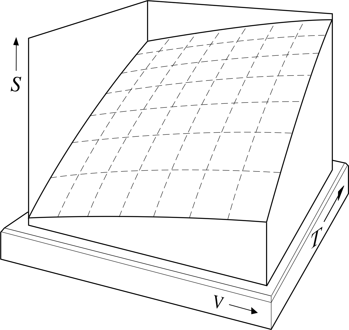
Figure 15 The SVT–surface for a fixed quantity of ideal gas.
Using Equation 46 (and Equation 19),
$\Delta Q = \frac32 nR\Delta T + P\Delta V$(Eqn 19)
we can see that the entropy of n moles of monatomic ideal gas occupying volume V at temperature T is given by
$S = \dfrac{3nR}{2}\loge\left(\dfrac{T}{T_0}\right) + nR\loge\left(\dfrac{V}{V_0}\right) + S_0$(47)
where S0 is a constant amount of entropy assigned arbitrarily to a state with volume V0 and temperature T0. The SVT surface for an ideal gas that corresponds to Equation 47 is shown in Figure 15. Different choices for the arbitrary constant S0, or for the reference state (V0, T0) to which it is assigned would raise or lower the whole surface, but would not distort one part relative to another.
✦ Using Equation 47, derive an expression for the difference in entropy between the equilibrium state of a n moles of ideal gas at temperature T1 and volume V1, and another state of the same gas, with temperature 2T1 and volume 2V1. Show that your answer does not depend on the values of V0, T0 or S0.
✧ For the first state, Equation 47,
$S = \dfrac{3nR}{2}\loge\left(\dfrac{T}{T_0}\right) + nR\loge\left(\dfrac{V}{V_0}\right) + S_0$(Eqn 47)
implies
$S_1 = \dfrac{3nR}{2}\loge\left(\dfrac{T_1}{T_0}\right) + nR\loge\left(\dfrac{V_1}{V_0}\right) + S_0$
and for the second state it implies
$S_2 = \dfrac{3nR}{2}\loge\left(\dfrac{T_2}{T_0}\right) + nR\loge\left(\dfrac{V_2}{V_0}\right) + S_0$
Subtracting the first equation from the second we see that
$S_2-S_1 = \dfrac{3nR}{2}\left[\loge\left(\dfrac{2T_1}{T_0}\right) - \loge\left(\dfrac{T_1}{T_0}\right)\right] + nR\left[\loge\left(\dfrac{2V_1}{V_0}\right) - \loge\left(\dfrac{V_1}{V_0}\right)\right]$
$\Delta S = \dfrac{3nR}{2}\left[\loge\left(\dfrac{2T_1}{T_1}\right)\right] + nR\left[\loge\left(\dfrac{2V_1}{V_1}\right)\right] = \dfrac{5nR}{2}\loge 2$
Thanks to the properties of logarithms, the final answer does not depend on T0 or V0, nor does it depend on S0.
5.3 The principle of entropy increase
In Subsection 5.1 we saw that in the context of a heat engine that absorbs heat Q1 at temperature T1, and rejects heat Q2 at temperature T2, a closed reversible cyclei occurs when
$\dfrac{Q_1}{T_1} = \dfrac{Q_2}{T_2}$(Eqn 43)
Since these heat transfers are isothermal processes we can use Equation 45,
$\Delta S = \dfrac{\Delta Q_{\rm rev}}{T}$ (isothermal case)(Eqn 45)
to say that the first of them increases the entropy of the system by an amount ∆S1 = Q1/T1 and the second decreases the entropy of the system by an amount ∆S2 = −Q2/T2. Note that we are using the symbol ∆S to represent a change in entropy, subject to the convention that a positive value of ∆S corresponds to an increase, and a negative value to a decrease.
It follows from Equation 43, that in a closed reversible cycle the total change in the entropy of the system is
$\Delta S_1 + \Delta S_2 = \dfrac{Q_1}{T_1} - \dfrac{Q_2}{T_2} = 0$(48)
In addition, we can carry out a similar analysis of the entropy changes in the environment. In particular, the first transfer will decrease the entropy of the environment so we can represent it by the negative quantity ∆S3 = −Q1/T1, while the second transfer will increase the entropy of the environment, so we can represent it by the positive quantity ∆S4 = Q2/T2. It then follows from Equation 43 that the total change in the entropy of the environment is
$\Delta S_3 + \Delta S_4 = \dfrac{-Q_1}{T_1} + \dfrac{Q_2}{T_2} = 0$(49)
It is clear from Equations 48 and 49 that the total change in the entropy of the universe (i.e. the system plus its environment) as a result of the full reversible cycle is zero. Moreover, because any change in the entropy of the system is always compensated by an opposite change in the entropy of the environment (e.g. ∆S1 + ∆S3 = 0), it is also true to say that over any part of a reversible cycle, even an infinitesimally small part, the total change in the entropy of the universe is zero.
This result is not confined to heat engines, in fact we can say generally that
Over any reversible process the entropy of the universe is unchanged:
$\displaystyle \int_i \Delta S_i = 0$(50)
However, what if a process is not reversible? The following example shows that in one case at least, an irreversible process leads to an increase in the entropy of the universe.
Example 3
A mass, m, of hot water at temperature TH is mixed in an insulating container with an equal mass of cold water at temperature TC. As a result of the mixing (an irreversible process) heat is transferred from the hot water to the cold water. Show that the overall effect of the process is to increase the entropy of the universe.
Solution
The heat lost from the hot water is equal to the heat gained by the cold water, both bodies of water have the same specific heat cP, and the same mass, so the final temperature of all the water will be
Tf = TH + TC/2
The heat exchanges occurring in the irreversible mixing may be quite complicated, but entropy is a function of state so the overall effect of those exchanges on the entropy can be determined by considering the effect of any reversible process that leads to the same final state. In this case a thermodynamically equivalent reversible process consists of placing each body of water into contact with a succession of thermal reservoirs of progressively higher (or lower) temperatures and at each stage allowing a small quantity of heat ∆Q to be transferred, causing a temperature change of ∆T, until the temperature Tf is reached. If the spacing ∆T between the temperatures of the thermal reservoirs is small enough each transfer of heat will be approximately isothermal and reversible, becoming exactly so in the infinitesimal limit.
The heat that must be reversibly transferred to cause an infinitesimal temperature change ∆T must then be mcP ∆T and we can use Equation 46 (which applies to reversible processes in general),
$\displaystyle \Delta S = S_{\rm b} - S_{\rm a} = \int_{\rm a}^{\rm b}\dfrac{\Delta Q}{T}$ (general case)Eqn (46)
to determine the total entropy change of the system:
$\displaystyle \Delta S = \Delta S_{\rm C} + \Delta S_{\rm H} = \int_{T_{\rm C}}^{T_{\rm f}}\dfrac{mc_PdT}{T} + \int_{T_{\rm H}}^{T_{\rm f}}\dfrac{mc_PdT}{T} = mc_P\left[\loge\left(\dfrac{T_{\rm f}}{T_{\rm C}} + \dfrac{T_{\rm f}}{T_{\rm H}}\right)\right]$
$\displaystyle \phantom{\Delta S } = mc_P\loge\left(\dfrac{T_{\rm f}^2}{T_{\rm C}T_{\rm H}}\right) = 2mc_P\loge\left(\dfrac{T_{\rm f}}{\sqrt{T_{\rm C}T_{\rm H}}}\right) = 2mc_P\loge\left(\dfrac{(T_{\rm H}+T_{\rm C})/2}{\sqrt{T_{\rm C}T_{\rm H}}}\right)$
You can see that ∆S > 0 for the system by choosing any values you like for TH and TC – the argument of the logarithmic function is always greater than 1 so the log is always positive. i There is no heat flow in or out of the system so the entropy of the environment does not change. Hence the increase in the entropy of the system also implies an increase in the entropy of the universe in this case.
Now, we have only considered one example of an irreversible process, but it illustrates a general result. A general analysis of irreversible processes, based on the second law of thermodynamics shows that
Over any irreversible process the entropy of the universe is increased:
$\displaystyle \int_i \Delta S_i \gt 0$(51)
Notice that entropy, unlike energy, is not generally a conserved quantity. Reversible processes conserve universal entropy but irreversible processes generate entropy, adding to the universal stock of that quantity.
Bringing Equations 50 and 51 together we have the statement known as
the principle of entropy increase
In any process, the entropy of the universe never decreases, so:
$\displaystyle \int_i \Delta S_{\rm universe} \ge 0$(52)
where the equality holds for reversible processes and the inequality for irreversible processes.
This is an extremely powerful and wide–ranging statement. It is really just another way of stating the second law of thermodynamics, so it may be used to derive the Clausius and Kelvin forms of the second law, and all of their consequences. This is a sufficiently important point that it merits an example.
Question T18
A thermal reservoir at a temperature of −20 °C is placed in thermal contact with another reservoir at 50 °C in such a way that 103 J of energy is transferred as heat from one reservoir to the other. Both reservoirs are totally isolated from the rest of the universe. Use the principle of entropy increase to show that the heat will flow from the hotter to the cooler body, in accordance with the Clausius form of the second law.
Answer T18
Thermal reservoirs absorb and reject heat isothermally and reversibly, so we can use Equation 45,
$\Delta S = \dfrac{\Delta Q_{\rm rev}}{T}$ (isothermal case)(Eqn 45)
to determine the entropy change that accepting or rejecting 103 J would have on each reservoir.
At the hotter reservoir ∆Saccept = 103 J/323 K = 3.10 J K−1 and ∆Sreject = −103 J/323 K = −3.10 J K−1.
At the cooler reservoir ∆Saccept = 103 J/253 K = 3.95 J K−1 and ∆Sreject = −103 J/253 K = −3.95 J K−1.
So, if the heat is accepted by the hotter reservoir and rejected by the cooler reservoir the entropy of the universe will change by −0.85 J K−1, but if the heat is rejected by the hotter reservoir and accepted by the cooler reservoir the change in universal entropy is +0.85 J K−1.
It follows from the principle of entropy increase, that the heat will flow from the hotter to the cooler body.
Question T19
10 g of steam at 100 °C condenses to water on a cold kitchen wall. Calculate the entropy change of the steam during the condensation. i
Does your answer contradict the second law of thermodynamics?
Answer T19
The latent heat released by the condensation is 10 g × 2.26 × 103 J g−1 = 2.26 × 10⁴ J. This energy will be transferred to the wall as heat, treating the transfer as isothermal and reversible, the change in the entropy of the steam will be ∆S = −2.26 × 10⁴ J/373K = −60.6 J K−1. This negative value does not contradict the principle of entropy increase or the second law of thermodynamics because the transfer of heat to the wall will lead to an increase in its entropy that more than compensates for the reduction in the entropy of the steam. The principle of entropy increase applies to the universe (i.e. system plus environment), not to the system alone.
The second law of thermodynamics predicts the direction of spontaneous change. This is especially clear when it is expressed in terms of the principle of entropy increase. The second law is quite unlike most other physical laws, which describe the relationships between quantities in a reversible process, without giving information about which must be ‘before’ and which ‘after’.
The second law also explains our intuitive feeling that systems somehow ‘lose’ energy, even though we know as physicists that energy is conserved. Hot objects cool down; moving objects spontaneously come to a stop. On the whole energy is not lost, but entropy is gained and the entropy of a system is a measure of the energy that is not available to do useful work. Any spontaneous ‘running down’ process is in fact irreversible; there is an increase in entropy and what is being ‘lost’ is not energy but the potential for further change.
5.4 The irreversibility of nature
The impossibility of reducing the entropy of the universe explains why naturally occurring processes happen in the way that they do, but it does not explain why such processes occur in the first place. The second law ensures that when heat flows spontaneously between bodies at different temperatures the flow will be from the hotter to the colder, but why should there be any flow at all? Neither the conservation of energy, nor the principle of entropy increase would be violated if the hot body stayed hot and the cold body stayed cold. The principle of entropy increase forbids a reduction in universal entropy, but the universe behaves as though some other principle demanded the maximum possible increase of entropy. What is it that underlies the spontaneity of the universe and gives it this appearance of actively striving for increased entropy? To gain some insight into this matter let us consider another example of an irreversible process.
Figure 16 A vessel in which a gas expands freely.
Example 4
An ideal gas, initially confined to a small volume Vi within a large vessel of volume Vf, is released and allowed to expand freely into the vacuum that fills the greater part of the vessel (Figure 16). Supposing that the vessel has rigid walls (ensuring that ∆W = 0), and is made of a heat insulating material (so ∆Q = 0), what is the change in universal entropy as a result of the expansion?
Solution
In this case the first law of thermodynamics implies that ∆U = ∆Q − ∆W = 0 and therefore ∆T = 0. As far as the system itself is concerned, the change in entropy may be deduced from Equation 47 as was shown in Subsection 5.2. The result is
$S_{\rm f} - S_{\rm i} = nR\loge\left(\dfrac{V_{\rm f}}{V_{\rm i}}\right)$
Due to the nature of the vessel there is no change to the entropy of the environment, so this expression which will always be positive, also represents the change in the entropy of the universe.
We can also interpret the irreversibility of the free expansion microscopically in terms of the movement of the gas molecules. All of the possible arrangements of the molecules while confined, are just a small proportion of the arrangements that are possible when the gas can occupy the full volume of the vessel. If all of these arrangements are equally likely, it is much more probable that the gas will be found to occupy the whole vessel rather than part of it. No thirst for entropy is required to achieve this, simply an unbiased exploration of all possible microscopic arrangements in a situation where the overwhelming majority of those arrangements involve filling the whole vessel.
The flow of heat from a hot body to a colder one can be explained in a similar way. The number of ways of distributing the energy of the bodies so that one has a higher temperature than the other is much less than the number of microscopic arrangements that correspond to both bodies having the same temperature. Thus a pointless exploration of accessible states once again explains an apparent striving for equilibrium.
What has this to do with the tendency of entropy to spontaneously increase rather than to remain unchanged? In his pioneering investigations of statistical mechanics the great Austrian physicist Ludwig Boltzmann (1844–1906) identified the entropy S of an isolated system as a measure of the number W of microscopic states available to that system. According to Boltzmann
S = k log W
where k = 1.381 × 10⁻²³ J K−1 is now known as Boltzmann’s constant.
The condition of thermal equilibrium is that in which the number of microstates in a closed system is maximized and is therefore also the one that maximizes the entropy. Spontaneous processes will therefore always tend to increase the entropy of the universe bringing it ever closer to overall thermal equilibrium.
6 Closing items
6.1 Module summary
- 1
-
Heating a substance may produce a rise in temperature or a phase transition. If there is no phase change, then the heat ∆Q needed to bring about a rise in temperature ∆T is proportional to the mass m of the sample and its specific heat c, with
∆Q = mc∆T(Eqn 2)
- 2
-
During a phase transition, a pure substance may absorb (or give out) heat with no change in temperature. If a mass m changes phase when heat ∆Q is supplied at constant temperature, then ∆Q = ml, where l is the specific latent heatof the substance. There are different latent heats for the processes of fusion (melting), vaporization (boiling) and sublimation (the direct conversion of a solid into a gas). Those latent heats also depend on the precise conditions under which the phase transition takes place.
- 3
-
Measurement of specific heats and latent heats involves supplying a known amount of heat and measuring its effect. Heat losses can be eliminated from the calculation by arranging for two different runs of an experiment to have the same heat losses.
- 4
-
The specific and latent heats of a substance depend on the constraints applied during heating. The principal specific heats are those measured at constant pressure and at constant volume.
- 5
-
For an ideal gas which satisfies
PV = nRT(Eqn 11)
the difference in principal molar specific heats is
CP − CV = R(Eqn 23)
and the ratio of specific heats
γ = CP /CV(Eqn 28)
depends on the nature of the gas molecules.
- 6
-
Common constraints applied to changes of state are characterized as isobaric (P = constant) isochoric (V = constant) isothermal (T = constant) and adiabatic (∆Q = 0). An ideal gas undergoing a quasistatic adiabatic process obeys the condition
PVγ = constant(Eqn 37)
where the constant is characteristic of the process.
- 7
-
Quasistatic processes may be represented as lines on a PVT–surface. On such a surface, the triple-point line marks the unique combination of pressure and temperature at which all three phases of a given sample of matter exist in equilibrium for a range of volumes. The critical point is the unique combination of pressure, temperature and volume at which liquid and vapour phases of a given sample are indistinguishable.
- 8
-
The Clausius–Clapeyron equation relates the slope of the boundary curve between two phases to the latent heat and change of volume involved in an isothermal crossing of that boundary
$\dfrac{dP}{dT} = \dfrac{ml}{T\Delta V}$(Eqn 40)
- 9
-
The Subsection 5.1second law of thermodynamics states that no process is possible whose sole result is the transfer of heat from a colder to a hotter body, or equivalently, that no process is possible in which the sole result is the transfer of heat from a body and its complete conversion into work.
- 10
-
The entropy of a system is a function of its state. The difference in entropy between two states a and b is given by
$\displaystyle \Delta S = S_{\rm b} - S_{\rm a} = \int_{\rm a}^{\rm b}\dfrac{\Delta Q}{T}$ (general case)(Eqn 46)
a where the integral may be evaluated over any reversible process that leads from state a to state b. If the two states are joined by a reversible isothermal process involving heat transfer ∆Q at temperature T
$\Delta S = \dfrac{\Delta Q_{\rm rev}}{T}$(Eqn 45)
For an ideal gas
$S = \dfrac{3nR}{2}\loge\left(\dfrac{T}{T_0}\right) + nR\loge\left(\dfrac{V}{V_0}\right) + S_0$(Eqn 47)
The entropy transferred in a process provides a measure of the extent to which energy transferred in that process is not available to do useful work.
- 11
-
According to the Subsection 5.3principle of entropy increase, in any process, the entropy of the universe never decreases. More precisely,
∆Suniverse ≥ 0(Eqn 52)
where the equality holds for reversible processes and the inequality for irreversible processes.
- 12
-
Processes that occur spontaneously are those which lead to an increase in the entropy of the universe.
6.2 Achievements
Having completed this module, you should be able to:
- A1
-
Define the terms that are emboldened and flagged in the margins of the module.
- A2
-
Calculate and use specific and latent heats.
- A3
-
Appreciate the advantage of having the same heat losses in two different runs of a calorimetry experiment.
- A4
-
Appreciate that the constraints applied to a system can affect the measurement of specific heat.
- A5
-
Solve problems in which an ideal gas undergoes quasistatic isothermal, adiabatic, isochoric or isobaric processes.
- A6
-
Recognize and use the values of the ratio of specific heats that typify an ideal monatomic and ideal diatomic gas.
- A7
-
Sketch and interpret quasistatic paths on a PVT–surface and on its P−V and P−T projections.
- A8
-
Identify the critical point, triple point, and triple–point line on a PVT–surface or its projections, and describe their physical significance.
- A9
-
Calculate entropy changes of a system and of its environment in sufficiently simple cases.
- A10
-
Describe the connection between the entropy change of the universe and the reversibility or otherwise of a process.
Study comment You may now wish to take the following Exit test for this module which tests these Achievements. If you prefer to study the module further before taking this test then return to the topModule contents to review some of the topics.
6.3 Exit test
Study comment Having completed this module, you should be able to answer the following questions each of which tests one or more of the Achievements.
Question E1 (A2)
Consider the mixing of hot water, cold water, and bath foam, with constant heat capacities m1c1, m2c2, m3c3 and initial temperatures T1, T2, T3. Derive an expression for the final temperature Tf after they have come to equilibrium (assuming no heat losses to the bathroom).
Answer E1
The equation which ensures that no heat is lost is
m1c1(Tf − T1) + m2c2(Tf − T2) + m3c3(Tf − T3) = 0
and this can be rearranged to give
$T_{\rm f} = \dfrac{m_1c_1T_1 + m_2c_2T_2 + m_3c_3T}{m_1c_1 + m_2c_2 + m_3c_3}$
(Reread Subsections 2.2 and 2.4 if you had difficulty with this question.)
Question E2 (A2, A4 and A6)
Gas is passed at constant pressure through a thermally–insulated tube containing an electric heater. A mass 5.4 g of gas flows into the tube in 90 s and, when the heater power is 0.16 W, the temperature difference between the outlet and inlet is 2.5 K. Calculate a value for the specific heat of the gas at constant pressure. Assuming this is a diatomic ideal gas, what is its specific heat at constant volume?
Answer E2
In 90 s the heat delivered is 0.16 W × 90 s = 14.4 J.
However,
$c_P = \dfrac{\Delta Q}{m\Delta T} = \rm \dfrac{14.4\,J}{5.4\times10^{-3}\,kg\times2.5\,K} = 1.07\,kJ\,kg^{-1}K^{-1}$
For a diatomic gas, cV = 5cP /7, so in this case
cV = 0.76 kJ kg−1 K−1
(Reread Subsections 2.2, 2.4 and 3.3 if you had difficulty with this question.)
Question E3 (A2 and A3)
In an experiment to determine the specific latent heat of vaporisation of benzene, it was found that when the electrical power input to the heater was 82 W, 10 g of benzene was evaporated in 1 min; when the power input was reduced to 30 W, the rate of evaporation was 2.0 g min−1. What is the advantage of doing two different runs of this experiment? Calculate the specific latent heat of vaporization of benzene.
Answer E3
Using the notation of Subsection 2.4, we have $\dot{Q} = \dot{m}l + \dot{H}$
We may assume that since both experiments are done at the same temperature (i.e. the boiling point of benzene) the heat lost in 1 minute will be the same in both cases. We thus have:
$82\,{\rm W} = \dot{H} + \dfrac{10\times10^{-3}\,{\rm kg\,min^{-1}}}{60\,{\rm s\,min^{-1}}}l$
and$30\,{\rm W} = \dot{H} + \dfrac{2\times10\times10^{-3}\,{\rm kg\,min^{-1}}}{60\,{\rm s\,min^{-1}}}l$
Subtracting one equation from the other we find l = 390 kJ kg−1.
(Reread Subsections 2.3 and 2.4 if you had difficulty with this question.)
Question E4 (A7 and A8)
Sketch a P–T plot showing the triple point and a P–V plot showing the critical point. Describe briefly the significance of these two points. What is the ‘triple-point line’?
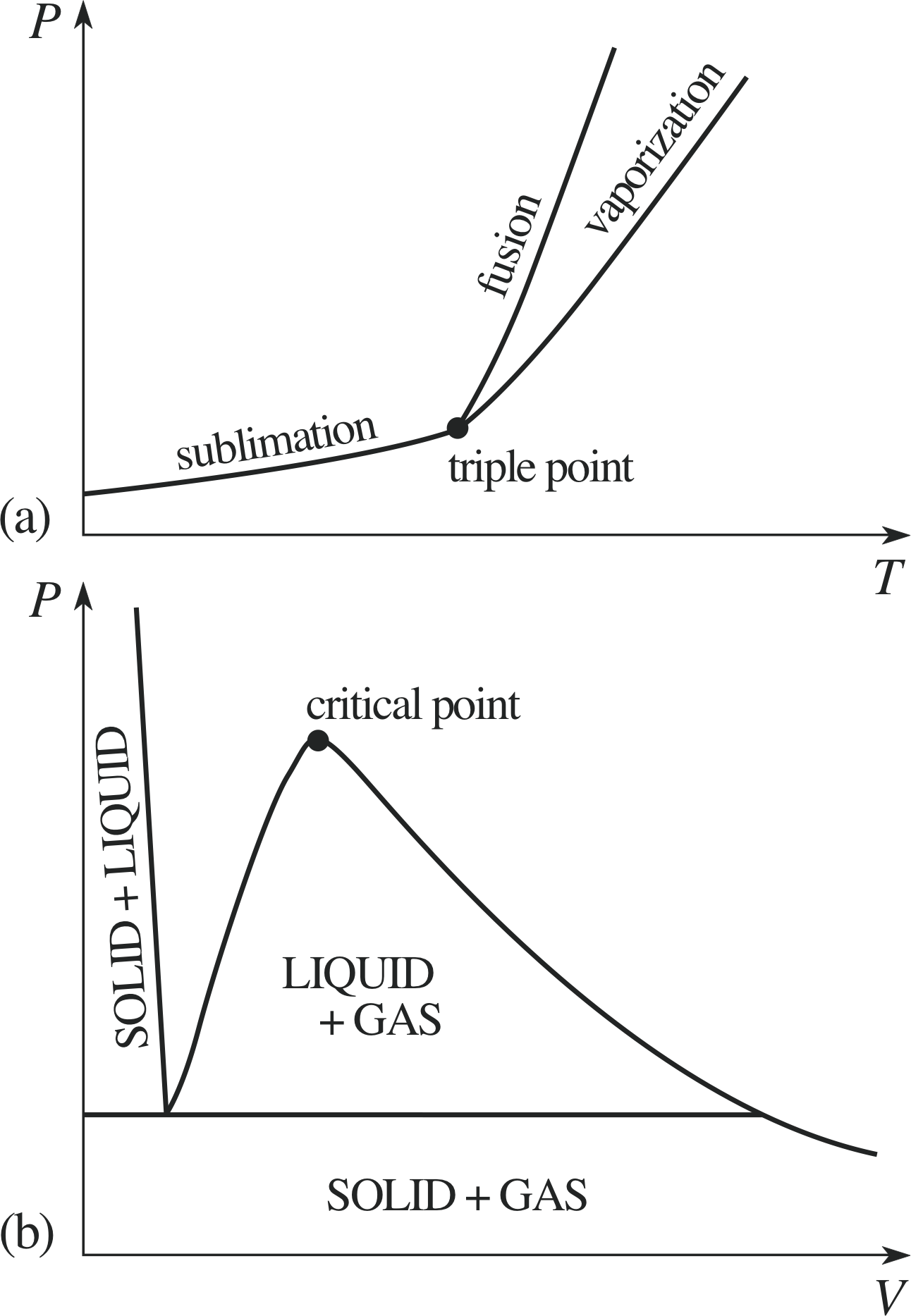
Figure 21 See Answer E4.
Answer E4
The P–T and P–V plots are shown in Figures 21a and b, respectively.
The triple point marks the combination of temperature, pressure and density (or molar volume) where three phases of a substance can coexist in equilibrium.
The triple–point line is a straight line parallel to the volume axis; it spans the finite range of volumes which a three–phase sample may have. The critical point marks the unique combination of temperature, pressure and density at which liquid and vapour phases are indistinguishable. It lies on the isotherm marking the maximum temperature at which the gas can be liquefied by isothermal compression.
(Reread Subsections 4.1, 4.2 and 4.3 if you had difficulty with this question.)
Question E5 (A2, A5 and A9)
A mass 5.0 × 10⁻⁴ kg of a certain vapour just becomes saturated when compressed to a volume V1 = 9.0 × 10⁻⁵ m3 and pressure 6.0 × 10⁶ Pa at a temperature 20°C. After isothermal compression to a volume V2, the substance is changed completely to liquid. The specific latent heat of vaporization of the liquid at 20°C is 1.2 × 10⁵ J−1. If V2 is negligible compared with V1, calculate:
(a) the work done during the compression from V1 to V2 and
(b) the heat supplied to, or removed from, the substance during compression.
(c) the changes in internal energy and in entropy of the fluid (i.e. a liquid + gas system).
Answer E5
The volume change ∆V is essentially 9.0 × 10⁻⁵ m3. The vapour pressure P remains constant at 6.0 × 10⁶ Pa during the compression.
(a) The work done on the fluid is P∆V = 6.0 × 106 Pa × 9.0 × 10−5 m3 = 540 J.
(b) The heat released by the fluid is ∆Q = ml = 5.0 × 10−4 kg × 1.2 × 105 J kg−1 = 60 J.
(c) From the first law of thermodynamics (Equation 4),
∆Q = ∆U + ∆W(Eqn 4)
∆U = ∆Q − ∆W = −60 J − (−540 J) = 480 J.
The fluid gives up heat reversibly at constant temperature and therefore
$\Delta S = \dfrac{\Delta Q}{T} = \rm \dfrac{-60\,J}{293\,K} = -0.205\,J\,K^{-1}$
(Reread Subsections 2.3 and 5.2 if you had difficulty with this question.)
Question E6 (A2, A9 and A10)
(a) Calculate the entropy change of the universe when:
(i) A copper block of heat capacity 150 J K−1 at 100°C is placed in a large lake at 10°C. (If you are unfamiliar with the techniques of integration you should consult Example 3 in Subsection 5.3 in answering this question.)
(ii) Two copper blocks at 100°C and 10°C, each of heat capacity 150 J K−1, are placed in thermal contact with each other and isolated from their environment.
(b) Comment on the reversibility or otherwise of these changes.
Answer E6
(a)
(i) From Equation 46,
$\displaystyle \Delta S = S_{\rm b} - S_{\rm a} = \int_{\rm a}^{\rm b}\dfrac{\Delta Q}{T}$ (general case)(Eqn 46)
and Example 3 in Subsection 5.3,
$\displaystyle \Delta S_{\rm copper} = \Delta S = \int_{T_{\rm i}}^{T_{\rm f}}\dfrac{mc_P}{T} = mc_P\loge\left(\dfrac{T_{\rm f}}{T_{\rm i}}\right) = \rm 150\,J\,K^{-1}\times\loge\left(\dfrac{283\,K}{373\,K}\right) = -41.4\,J\,K^{-1}$
As the copper block cools, the lake receives heat
∆Q = mccopper∆Tcopper = 90 K × 150 J K−1
Therefore∆Slake = ∆Q/Tlake = 90 × 150 J/283 K = 47.7 J K−1
and∆Suniverse = (47.7 − 41.4) J K−1 = 6.3 J K−1
(ii) The final temperature of the pair will be 55°C. The entropy change for each block as calculated as in part (i), and the net result is
$\rm 150\,J\,K^{-1}\times\left[\loge\left(\dfrac{55+273}{100+273}\right)+\loge\left(\dfrac{55+273}{10+273}\right)\right] = 150\,J\,K^{-1}\times(-0.129+0.148) = 2.85\,J\,K^{-1}$
(b) Neither change is reversible. They are both spontaneous changes and in each case there is a net increase in the entropy of the universe.
(Reread Subsections 2.2, 5.2, 5.3 and 5.4 if you had difficulty with this question.)
Study comment This is the final Exit test question. When you have completed the Exit test go back and try the Subsection 1.2Fast track questions if you have not already done so.
If you have completed both the Fast track questions and the Exit test, then you have finished the module and may leave it here.
Alternatively, you may wish to see the following section entitled Further reading.
7 Further reading
The following books all contain much more material than this module, so use each book’s index to locate the appropriate sections.
Thermal Physics by C. B. P. Finn (second edition published by Chapman and Hall, London, UK, 1993). Physics for Scientists and Engineers by R. A. Serway (second edition published by Saunders College, Philadelphia, USA, 1986).
Equilibrium Thermodynamics by C. J. Adkins (third edition published by Cambridge University Press, 1983).
Study comment Having seen the Fast track questions you may feel that it would be wiser to follow the normal route through the module and to proceed directly to the following Ready to study? Subsection.
Alternatively, you may still be sufficiently comfortable with the material covered by the module to proceed directly to the Section 6Closing items.