PHYS 7.5: Kinetic theory – an example of microscopic modelling |
PPLATO @ | |||||
PPLATO / FLAP (Flexible Learning Approach To Physics) |
||||||
|
1 Opening items
1.1 Module introduction
Modern physics tries to understand matter at a microscopic level, where bulk properties are explained in terms of atoms or molecules behaviour. One such theory is the kinetic theory which attempts to explain the bulk properties of gases in terms of a microscopic picture of the motion of atoms and molecules, interacting according to Newton’s laws of motion.
It is not feasible to attempt to apply Newton’s laws to each atom, since even a small macroscopic system of a few grams involves of the order of 1023 atoms. Not only would the mathematical task of solving the equations be impossible, but even a minute uncertainty in the initial position and velocity of each individual atom would, after a very short time, produce a prediction which bore no resemblance to the real situation. To deal with these enormous numbers, we have to use statistical methods that describe the average behaviour of the atoms. These statistical methods are based on the idea that the individual motions of atoms are random. It is the combination of Newton’s laws (to describe the individual atomic behaviour) and statistical reasoning (to describe the average behaviour of many atoms) that makes up the study of kinetic theory.
Section 2 begins the study of kinetic theory by considering an ideal gas. This is an ‘idealization’ of a real gas (one to which real gases approximate quite closely) in which the molecules are assumed to be vanishingly small and to interact with each other only during collisions. Using simple statistical ideas the macroscopic properties of the gas such as temperature, pressure, internal energy and specific heat can all be related to average molecular motion and this allows relationships between the macroscopic properties, such as the ideal gas law, to be derived. This section concludes with a discussion of the characteristic distances between collisions, the mean free path, and the characteristic time between collisions, the mean free time, relating both to molecular size and the average speed of the molecules.
Section 3 considers how individual molecular speeds are distributed about the mean molecular speed. This can be characterized in terms of a probability distribution function, the Maxwell–Boltzmann speed distribution function. This function is quoted and discussed, but its derivation lies beyond the scope of FLAP. The discussion of the speed distribution leads to the identification of three characteristic speeds for the distribution – the most probable speed, the average speed and the root-mean-squared speed. The distribution of molecular kinetic energies can then be derived from the speed distribution. This section concludes with brief discussions of the experimental validation of the speed distribution, and some of the transport processes in gases, e.g. diffusion, viscosity and thermal conduction.
In Section 4 we consider refinements to the simplest model of the ideal gas so as to describe real gases more accurately. This is done by incorporating molecular excluded volumes and intermolecular forces. This leads us to the introduction and discussion of the van der Waals equation of state.
Study comment Having read the introduction you may feel that you are already familiar with the material covered by this module and that you do not need to study it. If so, try the following Fast track questions. If not, proceed directly to the Subsection 1.3Ready to study? section.
1.2 Fast track questions
Study comment Can you answer the following Fast track questions? If you answer the questions successfully you need only glance through the module before looking at the Subsection 5.1Module summary and the Subsection 5.2Achievements. If you are sure that you can meet each of these achievements, try the Subsection 5.3Exit test. If you have difficulty with only one or two of the questions you should follow the guidance given in the answers and read the relevant parts of the module. However, if you have difficulty with more than two of the Exit questions you are strongly advised to study the whole module.
Question F1
In the kinetic theory of ideal gases, it can be shown that $PV = \frac23N\langle\varepsilon_{\rm tran}\rangle$, where P is the pressure, V the volume, N the total number of atoms or molecules in the gas and $\langle\varepsilon_{\rm tran}\rangle$ the average translational kinetic energy per molecule. (a) Explain how this leads to a microscopic definition of absolute temperature.
(b) Calculate the mean translational kinetic energy per atom for an ideal monatomic gas at 295 K. (Boltzmann’s constant k = 1.381 × 10⁻²³ J K−1).
(c) Calculate the total internal energy of 5.00 moles of a diatomic gas with five degrees of freedom at 295 K (the molar gas constant R = 8.314 J K−1 mol−1).
(d) What is the molar specific heat at constant pressure for this gas?
Answer F1
(a) Since the ideal gas equation of state is PV = nRT, we can equate the right–hand sides of both these equations (i.e. with $PV = \frac23N\langle\varepsilon_{\rm tran}\rangle$) and write:
$nRT = \dfrac23N\langle\varepsilon_{\rm tran}\rangle = \dfrac23\dfrac{N_A}{R}\langle\varepsilon_{\rm tran}\rangle = \dfrac{2}{3k}\langle\varepsilon_{\rm tran}\rangle$
i.e.$T = \dfrac23\dfrac{nN_A}{nR}\langle\varepsilon_{\rm tran}\rangle = \dfrac23\dfrac{N_A}{R}\langle\varepsilon_{\rm tran}\rangle = \dfrac{2}{3k}\langle\varepsilon_{\rm tran}\rangle$
This provides a definition of the macroscopic temperature T in terms of the average of the microscopic translational kinetic energy.
(b) We just rearrange the equation from (a):
$\langle\varepsilon_{\rm tran}\rangle = \frac32kT = $1.5 × 1.381 × 10−23 J K−1 × 295 K = 6.11 × 10⁻²¹ J
Note that if we know the temperature, we do not need the number of moles (or atoms) to calculate the mean kinetic energy per atom; we would need that information to calculate the total internal energy.
(c) For five degrees of freedom, the equipartition of energy theorem states that the internal energy will be $\frac25NkT{\text or }\frac25nRT$. So
$E_{\rm int} = \rm \dfrac25\times5\,mol\times8.314\,J\,K^{-1}\,mol^{-1}\times295\,K = 3.07\times10^4\,J$
(d) The specific heat at constant pressure is given by
$C_P = C_V + R = \frac52R + R = \frac72R = \rm \frac72\times8.314\,J\,K^{-1}\,mol^{-1} = 29.10\,J\,K^{-1}mol^{-1}$
Question F2
The Maxwell–Boltzmann speed distribution in a gas can be described by the equation:
$n(\upsilon)\Delta\upsilon = 4πN\left(\dfrac{m}{\pi kT}\right)^{3/2}\upsilon^2{\rm exp}(-m\upsilon^2/2kT)\Delta\upsilon$
where m is the atomic mass, k is Boltzmann’s constant, T the absolute temperature, N the number of molecules and υ the molecular speed.
(a) Explain briefly what this equation represents.
(b) One characteristic of the distribution is the root-mean-squared (rms) speed, given by:
$\upsilon_{\rm rms} = \sqrt{\dfrac{3kT}{m}}$
If the gas is molecular hydrogen (H2), one mole of which has a mass of 2.02 g, and the temperature is 250 K, what is the rms speed? (Avogadro’s constant NA = 6.02 × 10²³ mol−1, Boltzmann’s constant k = 1.381 × 10⁻²³ J K−1).
(c) Suppose you have two systems, one consisting of molecular hydrogen and the other of molecular oxygen. If their rms speeds are the same, what can you conclude about the relative temperatures of the two gases?
Answer F2
(a) n (υ)∆υ represents the number of atoms (or molecules) in the gas which have speeds in the small range υ to (υ + ∆υ), so it gives information on how the population of atoms is distributed among the range of possible speeds. (The area under a graph of n (υ) against υ, over the entire range of speeds, will just be the total number of atoms in the gas.)
(b) The mass of one mole of molecular hydrogen is 2.02 g, which means that the mass of an individual hydrogen molecule (which is what m in the equation represents) is 2.02 g/(6.02 × 1023) = 3.36 × 10⁻²⁴ g = 3.36 × 10⁻²⁷ kg. Then:
$\upsilon_{\rm rms} = \rm \sqrt{\dfrac{3\times1.381\times10^{-23}\,J\,K^{-1}\times250\,K}{3.36\times10^{-27}\,kg}} = \sqrt{3.08\times10^6\,m^2s^{-2}} = 1.76\times10^3\,m\,s^{-1}$
(c) Since their root-mean-squared speeds are the same, but their masses are different, their temperatures must be
different as well. We can rewrite the equation as $T = \dfrac{m}{3k}\upsilon^2$, so the molecule with the larger mass will have the higher temperature. The oxygen will be hotter.
(Section 3 gives a fuller discussion of the Maxwell–Boltzmann distribution.)
Question F3
The van der Waals equation of state can be written:
$\left(P+ \dfrac{a}{(V_{\rm m}^2-b)}\right)(V_{\rm m}-b) = RT$
where a and b are constants, Vm is the volume per mole of gas, and the remaining variables have their usual meanings.
(a) Explain briefly the physical interpretation of the terms which make this different from the ideal gas equation of state.
(b) For a particular gas the constants have values of a = 2.30 × 10⁻² N m4 mol−2 and b = 2.70 × 10⁻⁵ m3 mol−1. If 0.200 moles of the gas have a volume of 1.50 × 10⁻⁴ m3 at a pressure of 5.00 × 10⁶ Pa, what is T?
(c) The gas expands at constant temperature to a volume of 4.50 × 10⁻⁴ m3. What is the new pressure in Pa (1 Pa = 1 N m−2)?
Answer F3
(a) There are two differences between this equation and the ideal gas equation of state. First, instead of P we have the quantity [P + (a/Vm)]. This correction to the ideal gas behaviour represents the effect of intermolecular interactions. (See Subsection 4.3 for a more detailed explanation.)
The second difference is replacing the volume Vm by the term (Vm − b). This is a correction for the finite size of the molecules (which are points in the ideal gas model) and accounts for the excluded volume arising from the volumes of all the other molecules. (See Subsection 4.2 for more detail.)
(b) We rearrange the equation slightly and substitute in the given values:
$T = \dfrac{( P + a/V_{\rm m}^2)(V_{\rm m}-b)}{R}$
$\phantom{T }= \rm \left[5.00\times10^6\,Pa + \dfrac{2.30\times10^{-2}\,N\,m^4\,mol^{-2}}{(7.50\times10^{-4}\,m^3\,mol^{-1})^2}\right]\times\left[\dfrac{(7.50×10^{-4}-2.70\times10^{-5})\,m^3\,mol^{-1}}{8.314\,J\,K^{-1}\,mol^{-1}}\right] = 435\,K$
(Make sure you understand the unit conversions above.)
(c) Again, we need to rearrange the equation to solve for P:
$P+\dfrac{a}{V_{\rm m}^2} = \dfrac{RT}{V_{\rm m}-b}$
i.e.$P = \dfrac{RT}{V_{\rm m}-b} - \dfrac{a}{V_{\rm m}^2}$
Now we substitute in the given values (remembering that Vm (per mole) is five times the given value of V ):
$P = \rm \dfrac{8.314\,J\,K^{-1}\,mol^{-1}\times438\,K}{2.25\times10^{-3}\,m^3\,mol^{-1}-2.70\times10^{-5}\,m^3\,mol^{-1}} - \left[\dfrac{2.30\times10^{-2}\,N\,m^4mol^{-2}}{(2.25\times10^{-3}m^3\,mol^{-1})^2}\right]$
$\phantom{P }= \rm \dfrac{3.64\times10^3\,J\,mol^{-1}}{2.22\times10^{-3}\,m^3\,mol^{-1}} - \left(\dfrac{2.30\times10^{-2}\,N\,m^4mol^{-2}}{5.06\times10^{-6}m^6\,mol^{-2}}\right)$
$\phantom{P }= \rm 1.64\times10^6\,J\,m^{-3}-4.55\times10^3\,N\,m^{-2} = 1.64\times10^6\,Pa$
Again, make sure you understand the unit conversions.
1.3 Ready to study?
Study comment In order to study this module you should have a clear understanding of the following terms: absolute temperature, atom, atomic_mass_unitatomic mass, atomic mass unit, conservation of energy, conservation of momentum, density, displacement, elastic collision, force, kinetic energy (translational_kinetic_energytranslational, rotational_kinetic_energyrotational and vibrational_kinetic_energyvibrational), mole, molecule, Newton’s laws of motion, potential energy, pressure, relative molecular mass, speed, velocity, volume and work. You should be familiar with vectors, components_of_a_vectorvector components and vector addition and also with calculuscalculus notation, although the only derivative used is of a quadratic function. Ability to manipulate simple algebraic equations, including exponential functions, is assumed. If you are uncertain about any of these terms, review them by reference to the Glossary, which will also indicate where in FLAP they are developed. The following Ready to study question will allow you to establish whether you need to review some of the topics before embarking on this module.
Question R1
A particle travels from the point x = 0 m to x = 5 m, where it strikes a wall at 90° to the x–axis and then rebounds to the starting point. It moves at a uniform speed throughout − except for a negligible time at the turnaround. The total travel time is 10 s.
(a) What is the average speed over the time?
(b) What is the average velocity over the time?
(c) If the particle has a mass of 3 kg, what is the average kinetic energy over the time?
(d) What is the average magnitude of its momentum over the time?
(e) What is the change in momentum during the turnaround?
(f) If the duration of the collision with the wall is ∆t, what is the average force exerted on the wall during the collision?
Answer R1
(a) The average speed $\langle\upsilon\rangle$ is calculated by taking the ratio of the total distance travelled to the total time taken:
$\langle\upsilon\rangle = \rm (5 + 5)\,m/10\,s = 1\,m\,s^{-1}$
(b) The average velocity is calculated by taking the ratio of the net displacement to the total time taken for the displacement. Here the net displacement is zero and so
$\langle\boldsymbol{\upsilon}\rangle = {\rm \langle0\rangle\,m/10 s}\text{, with }\lvert\langle\boldsymbol{\upsilon}\rangle\rvert = \rm 0\,m\,s^{-1}$
The average velocity is zero because the net displacement is zero since the particle returns to its starting point.
(c) The average kinetic energy is
$m\langle\upsilon^2\rangle/2 = \rm 3\,kg\times(1\,m\,s^{-1})^2/2 = 1.5\,J$
(d) For the average magnitude_of_a_vector_or_vector_quantitymagnitude of momentum, we take the product of the mass with the average speed:
$\langle p\rangle = m \times\langle\upsilon\rangle = 3\,kg\times1\,m\,s^{-1} = 3\,kg\,m\,s^{-2}$
(e) Taking the momentum to be positive in the initial direction of motion:
momentum before the turnaround = p1 = 3 kg m s−1 in the initial direction
momentum after turnaround = p2 = −3 kg m s−2 in the initial direction
momentum change for particle is (p2 − p1) = −6 kg m s−2 in the initial direction
(f) According to Newton’s second law of motion, the average force exerted on the wall is equal to the rate of change of momentum, so F = −(p2 − p1)/∆t = (6/∆t) kg m s−1 in the initial direction.
Consult the relevant terms in the Glossary for further details.
2 Kinetic theory of ideal gases
2.1 The ideal gas model i
The goal of the kinetic theory of gases is to understand the bulk (macroscopic) properties of gases in terms of the constituent atoms or molecules – that is, to develop a microscopic model of these properties. When a physicist develops a model for a phenomenon, the first attempt always involves as much simplification as possible, keeping only the essential physical attributes and minimizing the mathematical complication. Our attempt to understand thermal phenomena at the microscopic level begins with the simplest system. We anticipate that the interactions between gas molecules are much weaker than those between molecules in solids or liquids, because in a gas the molecules are much further apart. We hope that this may allow us to describe the behaviour of gas molecules without having to know or calculate the detailed microscopic forces involved. We will ignore these forces, except when molecules collide, and assume all collisions are elastic collisions, conserving total kinetic energy.
To simplify the model further we will describe real gases without regard to their detailed molecular structure. This approach seems reasonable since we know that the behaviour of many gases approximates that of an ideal gas, characterized by:
the ideal gas equation of state or ideal gas law
PV = nRT(1)
where P is the pressure, V the volume, n the number of moles of gas i and R the universal molar gas constant of magnitude R = 8.314 J K−1 mol−1 and T is the absolute temperature.
The first task for our microscopic model is to explain this ideal gas equation, i.e. to develop the kinetic_theory_of_ideal_gaseskinetic theory of an ideal gas. This we will do in Subsection 2.2, but first try the following question.
Question T1
An ideal gas is in a container of volume 2.00 m3, with a pressure of 2.00 × 10⁵ Pa at a temperature of 310 K. (The universal gas constant R = 8.314 J K−1 mol−1).
(a) How many moles of the gas are contained?
(b) If the gas is made up of hydrogen molecules (which have a relative molecular mass of 2.02), what is the density of the gas?
(c) Suppose the volume of the container increased by a factor of two, with the temperature remaining constant. What would the new pressure be?
Answer T1
(a) Using the ideal gas law, PV = nRT, we find:
$n = \dfrac{PV}{RT} =\rm \dfrac{(2.00\times10^5\,Pa)\times2.00\,m^3}{8.314\,J\,K^{-1}\,mol^{-1}\times310\,K}$
$\phantom{n }= \rm \dfrac{4.00\times10^5\,Pa\,m^3}{2.58\times10^3\,J\,mol^{-1}} = \dfrac{4\times10^5\,N\,m}{2.58\times10^3\,N\,m\,mol^{-1}} = 155\,moles$
(b) The mass (in grams) of one mole of any substance is equal to its relative molecular mass, so for molecular hydrogen this is 2.02 g. Thus, the system contains 2.02 g × 155 = 313 g = 0.313 kg. The mass density is then
$\rho = \dfrac MV = \rm \dfrac{0.313\,kg}{2.00\,m^3} = 0.157\,kg\,m^{-3}$
(c) We have PV = constant, so if V increases by a factor of 2, P must decrease by a factor of 2. Thus, the new pressure is 1.00 × 10² Pa.
2.2 The assumptions of the kinetic theory of an ideal gas
Since the ideal gas equation works well for most real gases, irrespective of whether the molecules are monatomic_ideal_gasmonatomic (single atom), diatomic_ideal_gasdiatomic (two atoms), or triatomic_ideal_gaspolyatomic (more than two atoms), it is likely that an adequate model can be based upon the simplest form of microscopic particle – a point particle.
Study comment From now on we will use the word ‘molecule’ as a general term to describe the constituent particles of all gases, whether they be individual atoms, or diatomic molecules or polyatomic molecules. At some stages we will have to distinguish between these possibilities.
Now we will set out the five basic assumptions on which we can base the simplest microscopic model for gas behaviour – these form the foundation of the kinetic theory model of an ideal gas.
Assumption 1 The ideal gas consists of a large number of identical molecules which are in high speed random motion.
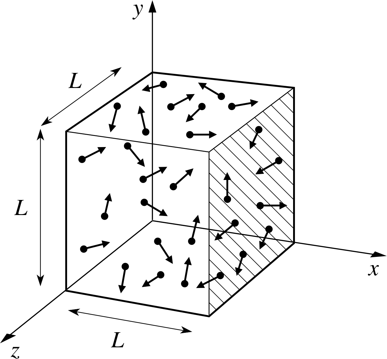
Figure 1 A schematic representation of the gas filled volume used in the kinetic theory calculation of pressure. The box contains N molecules, each with mass m. The direction of molecular motion (shown by the arrows) is random.
Implication Random motion means that the molecules are equally likely to be travelling in any direction. Although individual molecules undergo collisions and change direction frequently, the fact that there is a large number of them means that at any time there will be, to a very good approximation, equal numbers travelling in all directions, illustrated schematically in Figure 1. Molecules will also be uniformly distributed in space. i
Later we will discuss more implications of this randomness, but it is the crucial assumption of kinetic theory. We will use this randomness to discuss the properties of the gas in terms of the average molecule, which is all we will need to characterize much of the macroscopic behaviour of the gas.
Assumption 2 All molecular collisions, whether between molecule and molecule, or between molecule and wall, are elastic.
Implication You might guess that this is so since a gas isolated from external influences maintains its pressure and hence the molecules must maintain their kinetic energy. From this we can assume that kinetic energy must be conserved on a microscopic scale. You may be puzzled why perfectly elastic collisions are assumed between molecules, yet they never occur in the macroscopic world. The reason is that on a microscopic scale the walls also are molecular and these molecules are also in random vibrational motion. Therefore Assumption 2 implies that on average a molecule neither gains nor loses kinetic energy when it collides with another molecule – whether it is in the gas or in the wall.
Assumption 3 The molecular motion is governed by Newton’s laws of motion.
Implication We know today that quantum mechanics replaces the classical mechanics of Newton’s laws at the atomic level, but a classical model still gives many correct insights into the properties of gases. It is fortunate that the assumption that classical physics is applicable turns out to be justified in most of kinetic theory – there are only a few places where quantum mechanics is required, and we will point these out as we come to them.
Assumption 4 The molecules experience only contact forces. They interact like hard spheres and this only when they are in contact.
Implication We ignore the presence of long–range forces between the molecules (such as electrical forces). We can be fairly certain that some long–range forces exist, but ignoring them is reasonable if their magnitude is small. This assumption allows us to take the motions of molecules as being along straight lines between collisions.
Assumption 5 The volume occupied by the molecules themselves is very small compared to the volume occupied by the gas as a whole.
Implication This is another way of saying that the molecular diameter is small compared to the average distance between molecules and that the molecules may be treated as particles.
Question T2
(a) Using the ideal gas equation of state (Equation 1),
PV = nRT(Eqn 1)
calculate the volume occupied by one mole of an ideal gas at T = 300 K and at a pressure of 1.00 × 10⁵ Pa.
(b) Using the fact that the number of molecules per mole of gas is given by Avogadro’s constant NA (where NA = 6.02 × 10²³ mol−1), show that Assumption 5 is justified, taking a typical molecule as a sphere of radius r = 0.2 nm.
(c) What is the number of molecules per unit volume?
(d) If the average separation of the centres of these molecules in the gas is d, estimate d and compare this to the radius of a molecule.
Answer T2
(a) Using Equation 1,
PV = nRT(Eqn 1)
with n = 1 mol and R = 8.314 J K−1 mol−1, we find the volume of the gas
$V= \dfrac{nRT}{P} = \rm \dfrac{1\,mol\times8.314\,J\,K^{-1}mol^{-1}\times300\,K}{1.00\times10^5\,N\,m^{-2}} = 2.49\times10^{-2}m^3$
(b) The volume occupied by the molecules themselves is:
$N_A\left(\dfrac43\pi r^3\right) = \rm \dfrac{6.02\times10^{23}\,mol^{-1}\times4\times\pi\times(2\times10^{-10}m)^3}{3} = 2\times10^{-5}\,m^3\,mol^{-1}$
$\phantom{N_A\left(\dfrac43\pi r^3\right) }= 2\times10^{-5}\,{\rm m^3}\quad\text{for }n = 1\,{\rm mol}$
So, 1 mole of molecules occupies 2 × 10⁻⁵ m3, which is less than 0.1% of the total gas volume. Therefore Assumption 5 is justified.
(c) The number of molecules per unit volume is
$\dfrac{nN_A}{V} = \rm \dfrac{1\,mol\times6.02\times10^{23}\,mol^{-1}}{2.49\times10^{-2}m^3} = 2.42\times10 ^{25}\,m$
(d) If molecules have an average separation d, then each volume d3 contains on average one molecule.
Total gas volume V = nNAd3.
so$d^3 = \rm \dfrac{2.49\times10^{-2}m^3}{1\,mol\times6.02\times10^{23}\,mol^{-1}} = 2.49\times10^{-2}\,m^3$
and$d = \rm \sqrt[{\large3}\uproot{18}]{\dfrac{2.49\times10^{-2}}{6.02\times10^{23}}}\,m = 3.46\times10^{-9}\,m = 3.46\,nm$
The ratio $\dfrac dr = \rm \dfrac{3.46\times10^{-9}\,m}{0.2\times10^{-9}\,m} = 17$
So, the average molecular separation is 17 times the molecular radius.
Alternatively, we could have obtained the value for d3 from the answer to part (c). If the number of molecules per volume is x then
$d^3 = \dfrac{1}{x\os} = \rm \dfrac{1\,m^3}{2.42\times10^{25}}$
2.3 The molecular basis of temperature, pressure and internal energy
Before making detailed calculations let us consider what our model and our common experience qualitatively suggests about the temperature, pressure and internal energy of a gas. In general terms we may expect the internal energy of a system to increase as its temperature rises. For an ideal gas the only form of internal energy possible is the kinetic energy of the translational motion of its molecules. On this basis, we would expect the speed of our molecules to increase as the temperature of the gas increases. While we do not know the precise relationship, we would expect to be able to associate the molecular speed in some sense with the temperature, if our kinetic theory model is to make sense.
At the same level of understanding, the pressure exerted by the ideal gas must be the result of the collisions of the molecules with the walls of the container, so we would expect the pressure to increase as we add more molecules to the system or if we increase their speed by raising the temperature. This is in accordance with Equation 1,
PV = nRT(Eqn 1)
the pressure increases as the temperature increases for a fixed volume and a fixed number of moles of a gas; for a fixed temperature and volume, the pressure increases with the number of moles of gas.
On the basis of our simplified ideal gas point particle model, the molecules in the gas can have only translational kinetic energy. We might therefore associate the internal energy of a gas with the average translational kinetic energy per molecule. On the other hand, if the molecules have some internal structure, for instance if they are diatomic or polyatomic, then there could be additional energy associated with the rotational and vibrational motions of molecules For more complicated molecules, we might expect to associate the internal energy with the average total energy per molecule i, even though the temperature and pressure are associated with only translational kinetic energy. These are reasonable extensions to the simplified ideal gas point particle model, which allows no internal structure of the molecules.
These ideas about the molecular basis of temperature, pressure and internal energy are merely qualitative, but it is encouraging that the kinetic theory model seems to be consistent with our understanding of bulk properties at this level. However, for the model to be truly useful, we must be able to use it to make calculations, which in turn requires equations. These will be derived in the next subsection.
2.4 Kinetic theory and the ideal gas equation of state
Figure 1 A schematic representation of the gas filled volume used in the kinetic theory calculation of pressure. The box contains N molecules, each with mass m. The direction of molecular motion (shown by the arrows) is random.
We will derive the ideal gas equation of state (Equation 1),
PV = nRT(Eqn 1)
from the assumptions listed in Subsection 2.2, treating the molecules as point particles. We will start by using our kinetic theory model to calculate the pressure. The pressure is the net force exerted on unit area of the wall, so we need to calculate the force exerted by a molecule when it collides with the wall. The force exerted by the molecule on the wall is equal and opposite to the force exerted by the wall on the molecule, so we can work out either. The force on the wall at an impact can be calculated from Newton’s second law as the rate of change of momentum of the molecule. We take as our model a cubical box of side L, filled with N molecules each of mass m (see Figure 1). We will calculate the force exerted on the wall at x = L, shown by hatching on Figure 1.
Consider a typical molecule with velocity vector υ = (υx, υy, υz). Collisions of this molecule with the chosen wall arise because of the component υx and after the elastic wall collision υx is reversed, with υy and υz unchanged. Thus, if px represents the x–component of the molecule’s momentum and ∆px the change caused by a collision we can write:
initial value of px + ∆px = final value of px
i.e.mυx + ∆px = −mυx
so∆px = −mυx −(mυx) = −2mυx
Assuming no further intermolecular collisions, the molecule will return to impact on this wall again after rebounding from the wall at x = 0 – a round trip along x of length 2L that will require a time ∆t = 2L/υx. i The chosen molecule will therefore impact on the chosen wall once in each time interval ∆t, and from Newton’s second law, the average component of force in the x–direction $\langle f_x\rangle$ exerted by the wall, is given by the rate of change of momentum of the molecule in the x–direction, ∆px /∆t,
i.e.$\langle f_x\rangle = \dfrac{\Delta p_x}{\Delta t} = \dfrac{-2m\upsilon_x}{2L/\upsilon_x} = \dfrac{-m\upsilon_x^2}{L}$
This is the average force exerted by the wall on the molecule; the force exerted by the molecule on the wall will be just the negative of this. The effects of N molecules impacting on this same wall, each molecule with its own υx component, causes an average force $\langle F_x\rangle$ exerted on the wall given by:
$\langle F_x\rangle = -N\langle f_x\rangle = \dfrac{Nm}{L}\langle\upsilon_x^2\rangle$
where $\langle\upsilon_x^2\rangle$ is the average or mean squared υx component of all the N molecules,
i.e.$\displaystyle \langle\upsilon_x^2\rangle = \dfrac1N\sum_{i=1}^N\upsilon_{x_i}^2$ i
However, we want to know the pressure rather than the force, so we must divide the force by the wall area L2. The total pressure on the wall from the molecules is
$P_x = \dfrac{\langle F_x\rangle}{L^2}$
Substituting for $\langle F_x\rangle$ gives us
$P_x = \dfrac{Nm}{L^3}\langle\upsilon_x^2\rangle = \dfrac{Nm}{V}\langle\upsilon_x^2\rangle$(2)
where V is the volume of the gas. If we now invoke Assumption 1 we see that there is nothing special about our choice of x–axis – we could have reached similar conclusions about Py and Pz, so:
$P_y = \dfrac{Nm}{V}\langle\upsilon_y^2\rangle\quad\text{and}\quad P_z = \dfrac{Nm}{V}\langle\upsilon_z^2\rangle$
Assumption 1 implies
$\langle\upsilon_x^2\rangle = \langle\upsilon_y^2\rangle = \langle\upsilon_z^2\rangle$(3)
Thus Px = Py = Pz = P, where P is the pressure exerted by the gas, which is equal in all directions. The velocity components of an individual molecule are related to the speed υ by the expression:
υ2 = υx2 + υy2 + υz2
This relationship also must hold for the averages of these components and so the mean–squared speed is:
$\langle\upsilon^2\rangle = \langle\upsilon_x^2\rangle + \langle\upsilon_y^2\rangle + \langle\upsilon_z^2\rangle$
Equation 3 then gives
$\langle\upsilon_x^2\rangle + \langle\upsilon_y^2\rangle + \langle\upsilon_z^2\rangle = \frac13\langle\upsilon^2\rangle$(4)
You may have noticed that we have ignored collisions between molecules as they bounce back and forth between the walls. Surprisingly enough, this omission does not matter. The large number of molecules means that at any one time there will be as many molecules travelling towards the wall as away from it and because the collisions are elastic, the distribution of speeds will not vary with time (this is considered in more detail in Section 3). Thus the average effect on the wall will be the same as if the molecules never collided with each other.
Combining Equations 2 and 4 produces our required equation, which relates the macroscopic properties of a gas (on the left–hand side of Equation 5) and the average microscopic quantities (on the right–hand side of Equation 5):
$PV = \frac13Nm\langle\upsilon^2\rangle$(5)
Here $\langle\upsilon^2\rangle$ is the mean–squared speed of the molecules. The positive square root of this is known as the root_mean_square_r.m.s_speedroot–mean–squared (rms) speed υrms:
$\upsilon_{\rm rms} = \sqrt{\langle\upsilon^2\rangle}$(6)
So Equation 5 can be written as:
$PV = \frac13Nm\upsilon_{\rm rms}^2$
We can also write Equation 5 in terms of the aυerage molecular translational kinetic energy, $\langle\varepsilon_{\rm tran}\rangle$, i by noting that:
$\frac13m\langle\upsilon^2\rangle = \frac13\langle m\upsilon^2\rangle = \frac23\left\langle\frac12m\upsilon^2\right\rangle = \frac23\langle\varepsilon_{\rm tran}\rangle$
Equation 5 then becomes
$PV = \frac23N\langle\varepsilon_{\rm tran}\rangle$(7)
which relates the product PV to the average translational kinetic energy of the molecules in the gas. This is the result of our kinetic theory model calculation, and that is as far as we can take the equation simply on the basis of kinetic theory.
If you compare Equations 1,
PV = nRT(Eqn 1)
and Equation 7 you will see that the macroscopic ideal gas law and the kinetic theory result imply a particular association between temperature and the mean molecular kinetic energy. This relationship was anticipated qualitatively in Subsection 2.3. The relationship is:
$PV = nRT =\frac 2 N\langle\varepsilon_{\rm tran}\rangle$
or, taking the last two parts of the chain and rewriting them slightly we obtain:
$\langle\varepsilon_{\rm tran}\rangle = \dfrac32\dfrac{nR}{N}T = \dfrac32{nR}{nN_A}T = \dfrac32\dfrac{R}{N_A}T$(8)
where we have written the total number of molecules N in n moles as nNA, where NA is Avogadro’s constant, the number of molecules in one mole.
Equation 8 relates the macroscopic idea of absolute temperature to the average molecular (microscopic) translational kinetic energy of the molecules
$T = \dfrac23\dfrac{N_A}{R}\langle\varepsilon_{\rm tran}\rangle$(9)
Equation 9 gives us a microscopic definition of temperature in terms of the average molecular translational kinetic energy $\langle\varepsilon_{\rm tran}\rangle$.
Notice that the average molecular translational kinetic energy is determined only by the temperature and is independent of the molecular mass.
2.5 Boltzmann’s constant
Equation 8,
$\langle\varepsilon_{\rm tran}\rangle = \dfrac32\dfrac{nR}{N}T = \dfrac32{nR}{nN_A}T = \dfrac32\dfrac{R}{N_A}T$(Eqn 8)
is usually written as
$\langle\varepsilon_{\rm tran}\rangle = \frac32kT$(10)
where the new constant k, defined by the relationship
$k = \dfrac{R}{N_A}$(11)
is known as Boltzmann’s constant. i This constant appears frequently in equations relating macroscopic parameters to microscopic phenomena. From Equation 11 it is apparent that one can view k as the gas constant for one molecule in contrast with R, as the gas constant for one mole. The currently accepted value for k is 1.380 662 × 10−23 J K−1, normally rounded to 1.381 × 10⁻²³ J K−1.
We can express the root-mean-squared speed,
$\upsilon_{\rm rms} = \sqrt{\langle\upsilon^2\rangle}$(Eqn 6)
in terms of Boltzmann’s constant using Equation 10. Since m is a constant:
$\langle\varepsilon_{\rm tran}\rangle = \langle\frac12m\upsilon^2\rangle = \frac12m\langle\upsilon^2\rangle = \frac12m\upsilon_{\rm rms}^2 = \frac32kT$
i.e.$\upsilon_{\rm rms} = \sqrt{\dfrac{3kT}{m}}$(12)
Notice here that the root-mean-squared speed is determined by both the temperature and the molecular mass; this is in contrast to the average molecular kinetic energy which is determined only by the temperature.
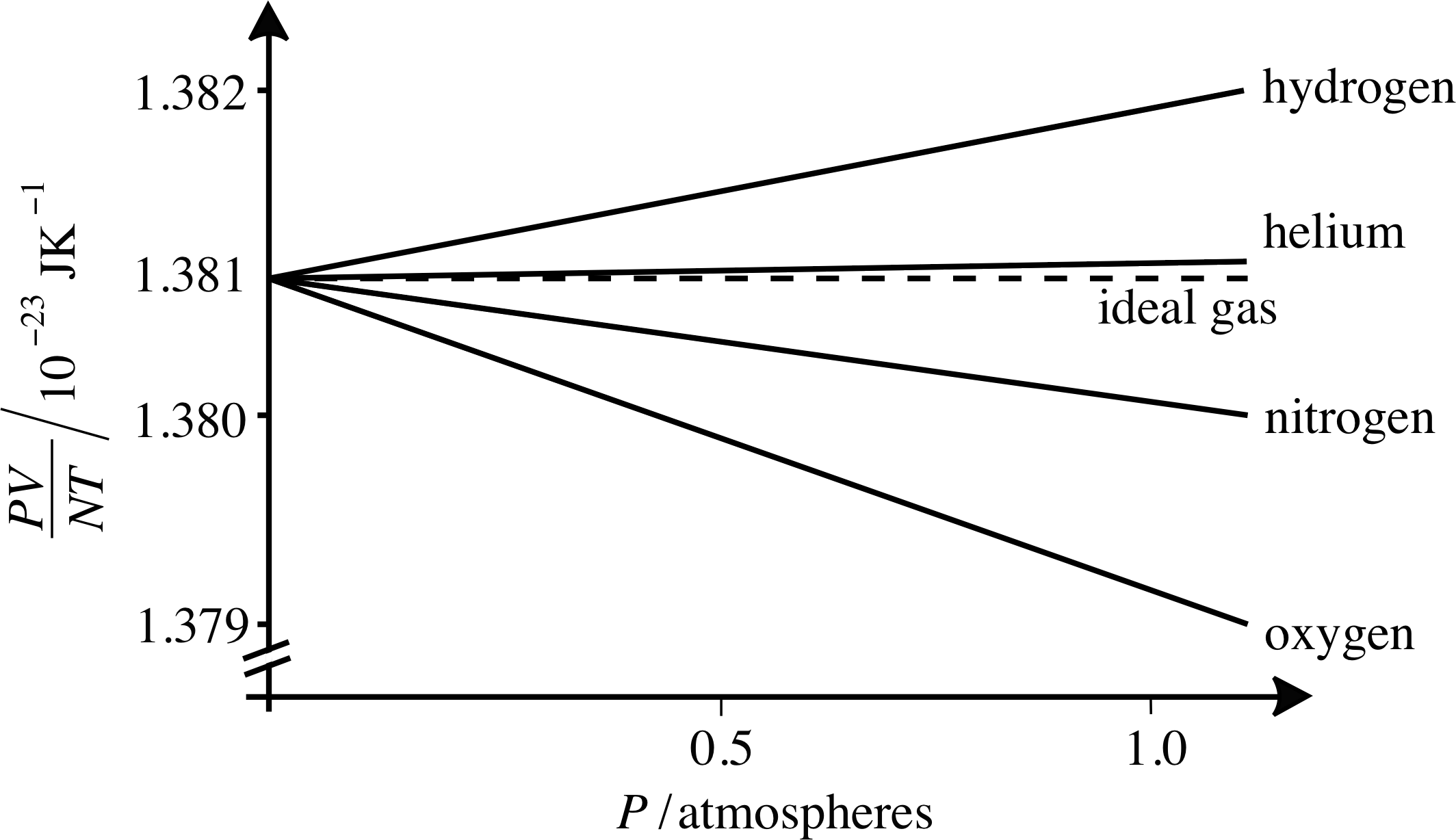
Figure 2 As the pressure falls towards zero, the value of PV/NT for all gases tends toward the ideal gas value, which is Boltzmann’s constant k. (Note the break in the vertical axis.)
Here k has arisen in relating the ideal gas law to kinetic theory. Another way of obtaining Boltzmann’s constant is by examining the behaviour of the quantity PV/NT as a function of pressure, as shown in Figure 2. Here we can see that as P approaches zero, the value of PV/NT approaches a single value for a range of simple gases, and that this number is Boltzmann’s constant. This is just what we would expect from the ideal gas law since PV = nRT = nNAkT. Thus the ideal gas law can be written as
PV = NkT(13)
with k = PV/NT.
Figure 2 also shows how real gases approach ideal gas behaviour at low pressures. As you can see from Figure 2, helium approximates better than others to the ideal gas law, but many more common gases deviate from this by no more than 0.1% even at atmospheric pressure.
Question T3
Calculate an average translational kinetic energy and a root-mean-squared speed for molecules of (a) helium (m = 6.6 × 10⁻²⁷ kg) and (b) argon (m = 6.6 × 10⁻²⁶ kg) each at a temperature of 300 K.
Answer T3
From Equation 9,
$T = \dfrac23\dfrac{N_A}{\varepsilon_{\rm tran}}$(Eqn 9)
for both gases
$\varepsilon_{\rm tran} = \rm \dfrac32\times\dfrac{8.314\,J\,K^{-1}mol^{-1}\times300\,K}{6.02\times10^{23}mol^{-1}} = 6.21\times10^{-21}\,J$
To calculate the speed, use Equation 12,
$\upsilon_{\rm rms} = \sqrt{3kT/m\os}$(Eqn 12)
For helium, m is 6.6 × 10⁻²⁷ kg, so:
$\upsilon_{\rm rms} = \rm \sqrt{\dfrac{3\times1.38\times10^{-23}\,J\,K^{-1}\times300\,K}{6.6\times10^{-27}\,kg}} = 1.37\,km\,s^{-1}$
For argon, m = 6.6 × 10⁻²⁶ kg, so υrms = 434 m s−1
Notice that although the average kinetic energies are the same, the helium atoms travel faster because they are
lighter.
Question T4
What gas temperature corresponds to an average molecular translational kinetic energy of 11electronvolt (1 eV = 1.6 × 10⁻¹⁹ J)?
What would be the root-mean-squared speed for H2 molecules (m = 3.3 × 10⁻²⁷ kg) at this temperature?
Answer T4
1 eV corresponds to an energy, in SI units, of 1.60 × 10⁻¹⁹ J.
From Equation 10,
For the monatomic gas $\langle \varepsilon_{\rm tran}\rangle = \frac32kT$(Eqn 10)
we have:
$T = \dfrac{2\langle\varepsilon_{\rm tran}\rangle}{3k} = \rm \dfrac{2\times1.6\times10^{-19}\,J}{3 \times1.38\times10^{-23}\,J\,K^{-1}} = 7.72\times10^3\,K$
For hydrogen molecules (m = 3.3 × 10⁻²⁷ kg), at this temperature, Equation 12,
$\upsilon_{\rm rms} = \sqrt{3kT/m\os}$(Eqn 12)
gives:$\upsilon_{\rm rms} = \rm \sqrt{\dfrac{3\times1.38\times10^{-23}\,J\,K^{-1}\times7.73\times10^3\,K}{3.3\,10^{-27}\,kg}} = 9.85\,km\,s^{-1}$
2.6 Kinetic theory and the internal energies of molecules
We have already shown that the pressure and temperature of an ideal gas are determined by the average translational kinetic energy of the molecules in the gas. If we allow our molecules only to be monatomic hard spheres (as we have done so far), then that is the only significant form the energy can take. However, if we allow for more complex diatomic or polyatomic molecules then energy may also be stored as kinetic and potential energy within individual molecules as a molecule can vibrate or rotate about its centre of mass. When energy is added to a sample of such a gas the translational motion of its molecules will increase, but also they may store some of this energy in additional rotational or vibrational motion. The total energy of such a molecule would exceed that due to translational motion alone. i
For the monatomic gas
$\langle\varepsilon_{\rm tran}\rangle = \frac23kT$(Eqn 10)
and we assumed that the molecules were free to move in three dimensions, but that they had no internal structure and hence no rotational or vibrational energy. This freedom to move in three dimensions can be expressed by saying that the molecules have three degrees of freedom. If we were to allow for rotational or vibrational motion then this would give additional degrees of freedom, in which additional energy may be present.
Where there are several degrees of freedom available statistical mechanics i leads to the result that, on average, the available energy will be shared equally between all degrees of freedom.
The proof of this lies beyond the scope of FLAP but it is another manifestation of the assumption of total randomness, and it is known as the equipartition of energy theorem.
The equipartition of energy theorem states that each degree of freedom possesses an average energy of ½ kT per molecule.
So, with three degrees of freedom each molecule has an average energy of $3\times\frac12kT = \frac23kT$ and this average total energy per molecule, $\langle\varepsilon_{\rm tot}\rangle$, is purely translational.
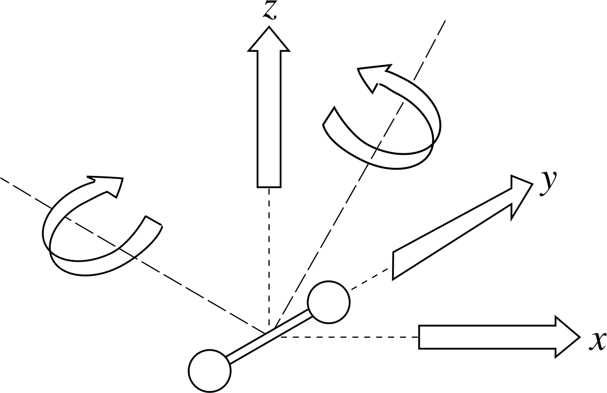
Figure 3 Five independent degrees of freedom (two directions of rotation and three of translation) for a dumbell–shaped diatomic molecule.
✦ Suppose our molecules are diatomic, with their atoms rigidly connected along a line and are unable to vibrate along this line. We can define two mutually perpendicular axes of rotation at right angles to this line and it can be shown that these count as two additional degrees of freedom i (see Figure 3). What is the average total energy per molecule in this case?
✧ We have three translational degrees of freedom plus two rotational degrees of freedom, giving a total of five. This means that the average total energy per molecule is
$\langle\varepsilon_{\rm tot}\rangle = \langle\varepsilon_{\rm tran}\rangle + \langle\varepsilon_{\rm rot}\rangle = \frac32kT + \frac22kT = \frac52kT$
In general, if a molecule has q degrees of freedom then:
$\langle\varepsilon_{\rm tot}\rangle = \dfrac q2\dfrac{R}{N_A}T = \dfrac q2kT$(14a)
or$T = \dfrac2q\dfrac{N_A}{R}\langle\varepsilon_{\rm tot}\rangle = \dfrac{2}{qk}\langle\varepsilon_{\rm tot}\rangle$(14b)
Equation 14b provides an alternative to Equation 9,
$T = \dfrac23\dfrac{N_A}{R}\langle\varepsilon_{\rm tran}\rangle$(Eqn 9)
as a microscopic definition of temperature.
We can now relate the total internal energy, Eint, for the whole molecular system to a key macroscopic parameter, the absolute temperature. For a gas of N molecules with q degrees of freedom, we can write
$E_{\rm int} = N\langle\varepsilon_{\rm tot}\rangle = \dfrac q2NkT$(15)
Question T5
Suppose that you have two gas samples, each of one mole, at the same temperature and pressure. One gas is monatomic and the other is diatomic, with the molecules able to rotate but not vibrate. i If the same amount of energy is added to each sample, which will reach the higher temperature?
Answer T5
For the two samples each containing one mole we have:
energy added = $\Delta E_{\rm int}$
energy added = $\frac32Nk(\Delta T)_{\rm monatomic}$
energy added = $\frac52Nk(\Delta T)_{\rm diatomic}$
where N = NA × 1 mol in each case, so
$(\Delta T)_{\rm diatomic} = \frac35(\Delta T)_{\rm monatomic}$
So the monatomic system reaches the higher temperature.
This is because in the monatomic molecule the temperature corresponds only to the amount of translational kinetic energy in the system; in the case of the diatomic molecule, the energy is shared out between translational and rotational kinetic energy.
2.7 Kinetic theory and the specific heat of gases
The specific heat is defined as the energy required to raise the temperature of a specified amount of material by one degree absolute. Normally the specified amount is 1 kg, with the specific heat measured in units of J K−1 kg−1. We can also define a molar specific heat, which has units of J K−1 mol−1, where the specified amount is one mole. From the general definition of specific heat we can define the molar specific heat by the equation:
$C = \dfrac{\Delta Q_{\rm m}}{\Delta T}$(16)
where C is the molar specific heat, ∆Qm is the energy supplied per mole of gas, in the form of heat, i causing a change in temperature ∆T. i For a gas, the conditions under which the energy is added must be carefully specified, (e.g. at constant pressure, or at constant volume), since this will affect the value of the resulting specific heat. We will consider now what our kinetic theory model for the ideal gas tells us about these specific heats.
First we will consider CV, the molar specific heat at constant volume. When heat is added to the system, the energy transferred to the gas must increase the energy of the gas molecules. This is all that can happen if the process is at constant volume. For a monatomic ideal gas, we therefore see from Equation 15,
$E_{\rm int} = N\langle\varepsilon_{\rm tot}\rangle = \dfrac q2NkT$(Eqn 15)
that the increase in internal energy corresponding to a temperature increase ∆T is
$\Delta E_{\rm int} = \dfrac32Nk\Delta T = \dfrac32nR\Delta T$
where n is the number of moles present. Thus, to cause the temperature rise, the heat that must be supplied per mole is
$\Delta Q_{\rm m} = \dfrac{\Delta E_{\rm int}}{n} = \dfrac32\dfrac{Nk\Delta T}{n} = \dfrac32R\Delta T$
so$C_V = \left(\dfrac{\Delta Q_{\rm m}}{\Delta T}\right)_V = \dfrac32N_Ak = \dfrac32R$(17) i
where R is the gas constant (Equation 11),
$k = \dfrac{R}{N_A}$(Eqn 11)
If we have polyatomic molecules with q degrees of freedom, this is simply generalized to:
$C_V = \dfrac q2N_Ak = \dfrac q2R$(18)
We also need to derive an expression for the molar specific heat at constant pressure, CP. The difference between the two specific heats, in terms of bulk properties, is that for the constant pressure process, the gas will expand as heat is added. This means that part of the energy transferred to the system as heat will be used to do the work of expansion and there will be a correspondingly smaller increase in internal energy than for the constant volume system. Since the internal energy of the ideal gas is proportional to the absolute temperature, there will be a smaller rise in temperature for the same amount of heat transferred, which implies that CP > CV. We will now try to understand this in terms of our kinetic theory model.
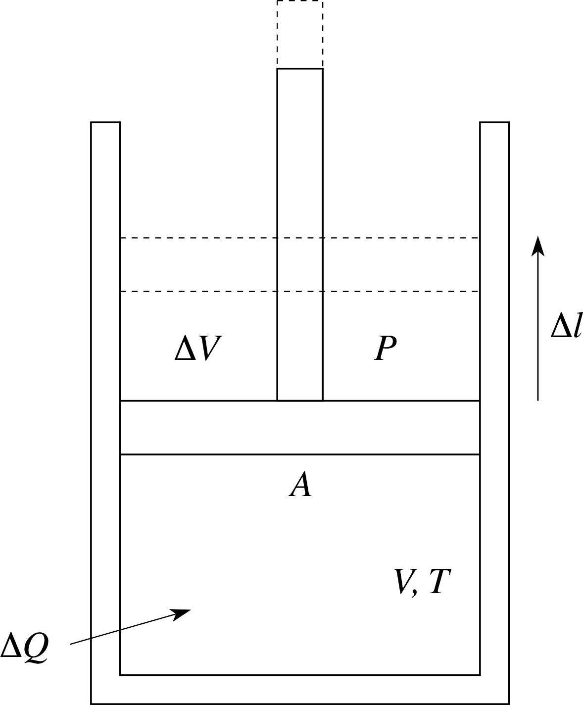
Figure 4 Expansion of a gas under constant pressure conditions.
As heat is added to the system, the volume increases to maintain constant pressure. This could be done by having the gas contained in a cylinder with a frictionless piston (see Figure 4), with a fixed reference pressure (say atmospheric pressure) on top of the piston. As the gas in the cylinder is heated, the piston will rise, maintaining constant pressure, so allowing the volume to increase. How can we interpret this microscopically?
In Subsection 2.4 we assumed that the wall of the container was held rigidly in place by external forces, so that the elastic collisions of the molecules caused no recoil of the wall itself. Now we are going to allow the wall of the piston to move in response to the collisions, by making the piston frictionless, so we need to re–analyse the situation. In an elastic collision where both masses are free to move, the energy will be shared out between them. This means that the molecules will, on average, transfer some of their kinetic energy to the recoiling piston as the gas expands and more heat will therefore be required to produce the same rise in temperature, compared to the constant volume case.
In Figure 4 the gas initially has volume V, pressure P, temperature T and is contained in a cylinder with a piston of cross–sectional area A. An amount of heat ∆Q is added to the gas, its temperature rises to (T + ∆T) and it also expands under constant pressure P to volume (V + ∆V). To raise the piston, the gas must apply an upwards force of magnitude F given by F = PA. The gas does work by raising the piston a distance ∆l.
This work done by the gas is given by
∆W = F∆l = PA∆l = P∆V
Using the principle of energy conservation
heat added = change in internal energy of gas + work done by the gas
we obtain the first law of thermodynamics:
∆Q = ∆Eint + P∆V(19) i
We can calculate P∆V from Equation 1,
PV = nRT(Eqn 1)
by considering the system before and after the expansion. For an ideal gas:
initiallyPV = nRT
and finallyP (V + ∆V) = nR (T + ∆T)
If we subtract these two, we find
P∆V = nR∆T(20)
∆Eint for the system can be obtained from Equation 15,
$E_{\rm int} = N\langle\varepsilon_{\rm tot}\rangle = \dfrac q2NkT$(Eqn 15)
and using Equation 18 we may write this as
∆Eint = nCV ∆T(21)
If we now substitute Equations 20 and 21 into Equation 19,
∆Q = ∆Eint + P∆V(Eqn 19)
and divide both sides by n we find that at constant pressure the heat per mole required to raise the temperature by ∆T is
∆Qm = CV ∆T + R∆T = (CV + R)∆T
so$C_P = \left(\dfrac{Q_{\rm m}}{\Delta T}\right)_P = C_V + R$ i
i.e.CP − CV = R(22)
Equation 22 gives the difference in the molar specific heats for an ideal gas. As expected from our earlier discussion, CP exceeds CV.
The ratio of the specific heats, CP /CV is often written as γ, i and using Equations 22 and 18,
$C_V = \dfrac q2N_Ak = \dfrac q2R$(Eqn 18)
we see that
$\gamma = \dfrac{C_P}{C_V} = 1 + \dfrac{R}{C_V} = 1 + \dfrac{R}{\dfrac q2R} = 1 + \dfrac2q$(23)
Notice that the difference between the two specific heats is independent of the number of degrees of freedom q of the molecule, but the two specific heats themselves and their ratio γ depend on q.
Question T6
How would the expression for the specific heat at constant pressure be generalized to the case of a polyatomic molecule with q degrees of freedom?
Answer T6
Using Equations 18 and 22,
$C_V = \dfrac q2N_Ak = \dfrac q2R$(Eqn 18)
CP − CV = R(Eqn 22)
we have the generalization:
$C_P = \dfrac q2R + R = \dfrac{q+2}{2}R$
We may collect the result from Question T6 into our set of equations by writing, for a gas with q degrees of freedom:
$C_P = \left(1 + \dfrac q2\right)R$(24)
Question T7
Predict the values of CV, CP, (CP − CV) and γ = CP /CV for gases having, (a) three degrees of freedom, (b) five degrees of freedom, (c) seven degrees of freedom.
Answer T7
The values for CV, CP, (CP − CV) and γ, as given in Table 2, are determined from Equations 18, 22, 23 and 24:
| q | CV = qR/2 | CP = (1 + q/2)R | (CP − CV) = R | γ = CP /CV = 1 + 2/q |
|---|---|---|---|---|
| 3 | 3R/2 | 5R/2 | R | 5/3 |
| 5 | 5R/2 | 7R/2 | R | 7/5 |
| 7 | 7R/2 | 9R/2 | R | 9/7 |
$C_V = \dfrac q2N_Ak = \dfrac q2R$(Eqn 18)
CP − CV = R(Eqn 22)
$\begin{align}\gamma & = \dfrac{C_P}{C_V} = 1 + \dfrac{R}{C_V}\\ & = 1 + \dfrac{R}{\dfrac q2R} = 1 + \dfrac2q\end{align}$(Eqn 23)
$C_P = \left(1 + \dfrac q2\right)R$(Eqn 24)
The conclusion from this subsection is that our microscopic kinetic theory model allows the number of degrees of freedom of the molecules in a gas to be inferred from macroscopic measurements of the gas specific heats.
2.8 The mean free path of an ideal gas molecule
In Subsection 2.4, it was claimed that intermolecular collisions did not invalidate the derivation of Equation 5,
$PV = \frac13Nm\langle\upsilon^2\rangle$(Eqn 5)
However, it is still of interest to know something about the frequency of these collisions and how far molecules travel between them.
The mean free path λ i of a molecule is defined as the average distance it travels between collisions. We might expect the mean free path to vary strongly with temperature and pressure as these properties determine the speed and the closeness of the molecules, respectively. We can get a feel for the kind of distances involved by thinking about a specific example. Let us consider one mole of a gas at a temperature of 300 K and a pressure of 1.0 × 10⁵ Pa – these were the conditions for the gas in Question T2.
✦ What is the number density (the number of molecules per unit volume) for molecules under these conditions?
✧ The number density will be N/V where N = number of molecules, V = volume. As there is one mole of gas, N = 6.02 × 10²³ and the volume can be calculated from the ideal gas equation V = nRT/P with n = 1 mol. From Answer T2 this volume is given as V = 2.49 × 10⁻² m3.
The number density nρ is given by
nρ = N/V = 2.42 × 1025 m−3 i
In Question T2 we calculated the average separation between molecules under these conditions as 3.46 nm. You might expect that the mean free path would be very similar to the intermolecular separation – in fact it is considerably different, as we will see in a moment – mainly because it also depends on the size of the molecules as well as on their mean separation.
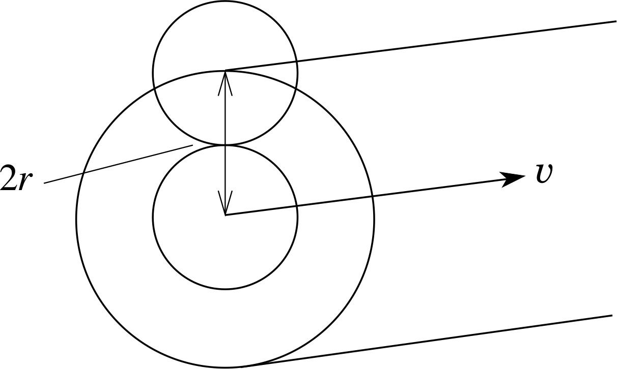
Figure 5 A molecule travelling through the gas sweeps out a volume that is cylindrical, with the axis coinciding with the centre of the molecule.
To calculate λ, we need to think about the average volume per molecule. This must also be the volume a molecule will have to sweep through before it makes a collision. A molecule will contact another identical molecule if (assuming they are spherical) the distance between their centres is equal to twice the molecular radius or 2r (see Figure 5).
We are only interested in centre-to-centre intermolecular distances, so the situation is equivalent to one where all the other molecules are considered to be points, and our reference molecule has a radius of 2r.
In a time ∆t our reference molecule, assumed to be travelling with the average speed $\langle\upsilon\rangle$, sweeps out a volume equal to that of a cylinder of length $\langle\upsilon\rangle\Delta t$ and radius 2r. This volume is $\Delta V = \pi(2r)^2\langle\upsilon\rangle\Delta t = 4\pi r^2\langle\upsilon\rangle\Delta t$. All other molecules whose centres lie within this volume will be struck by the reference molecule within the time ∆t. This number is nρ ∆V where nρ is the number density of the molecules. So, in a time ∆t the number of collisions with the reference molecule is $4\pi r^2n_\rho\langle\upsilon\rangle\Delta t$. We can define the mean collision frequency fcoll (mean number of collisions per second) as
$f_{\rm coll} = \dfrac{\text{mean number of collisions in }\Delta t}{\Delta t} = \dfrac{4\pi r^2n_\rho\langle\upsilon\rangle\Delta t}{\Delta t} = 4\pi r^2n_\rho\langle\upsilon\rangle$(25)
The mean time between collisions, or the mean free time τcoll i is
$\tau_{\rm coll} = \dfrac{1}{f_{\rm coll}} = \dfrac{1}{4\pi r^2n_\rho\langle\upsilon\rangle}$(26)
and the mean distance between collisions, or the mean free path λ, is
$\lambda = \langle\upsilon\rangle\tau_{\rm coll} = \dfrac{1}{4\pi r^2n_\rho}$(27)
Notice that the mean free path is independent of the average molecular speed. You may be concerned that this simple calculation has ignored the effects of collisions on our calculated volumes. Again we are justified in doing this because of Assumption 1. Since we are concerned with random motion, we only have to use averages. In fact, a more careful calculation, which takes into account the motion of all the molecules, changes these results only by a factor of 2, so that for example, the expression for mean free path becomes
$\lambda = \dfrac{1}{4\sqrt{2\os}\pi r^2n_\rho}$(28)
Question T8
Use Equation 28 to calculate the mean free path for the gas discussed in Question T2. (i.e. an ideal gas at T = 300 K and at a pressure of 1.00 × 10⁵ Pa. )
Answer T8
If we substitute the figures from Question T2 (i.e. an ideal gas at T = 300 K and at a pressure of 1.00 × 10² Pa) into Equation 28,
$\lambda = \dfrac{1}{4\sqrt{2\os}\pi r^2n_\rho}$(Eqn 28)
we find:
$\lambda = \rm \dfrac{1}{4\sqrt{2\os}\pi\,(2\times10^{-10})^2\,m^2\times2.42\times10^25\,m^{-3}} = 58\,nm$
This is equivalent to about 145 molecular diameters and is about 17 times the intermolecular separation.
Question T9
In Question T2 we estimated that the average separation between molecules (of diameter 0.4 nm) in this gas was about 3.5 nm (equivalent to 8.75 molecular diameters), but in Question T8 we have calculated a mean free path which is 58 nm (equivalent to 145 molecular diameters). Are these numbers consistent? Give your reasoning.
Answer T9
Yes, they are consistent.
The first estimate is that there will be another molecule within about 8.75 diameters in some direction, while the second value is estimating how far the molecule will have to travel in a particular direction before colliding with another molecule. The second value depends on the size of the targets but the first does not. For the mean free path, we are essentially asking how long a cylinder with twice the diameter of a molecule must be to have the same volume as the cube that, on average, contains one molecule.
2.9 Summary of Section 2
The kinetic theory model of an ideal gas is based on Newton’s laws and certain simplifying assumptions. The simplifying assumptions are as follows:
- Assumption 1
- The ideal gas consists of a large number of identical molecules in high speed random motion.
- Assumption 2
- All collisions between molecule and molecule, or between molecule and wall, are elastic.
- Assumption 3
- The individual molecules obey Newton’s laws of motion.
- Assumption 4
- The molecules only experience contact forces. They interact like hard spheres and this only when they touch.
- Assumption 5
- The volume occupied by the molecules themselves is very small compared to the volume occupied by the gas as a whole.
This model provides a derivation of the ideal gas equation of state (PV = nRT) and shows that the absolute temperature can be expressed in terms of the average kinetic energy per molecule:
$T = \dfrac23\dfrac{N_A}{R}\langle\varepsilon_{\rm tran}\rangle = \dfrac{2}{3k}\langle\varepsilon_{\rm tran}\rangle$(Eqns 9 and 10)
Boltzmann’s constant is a useful parameter, it is defined by the equation k = R/NA and can be interpreted as the gas constant per molecule.
The kinetic theory model can be used to derive theoretical expressions for the specific heat of an ideal gas at constant volume and at constant pressure and for the mean free path of a molecule. In a monatomic ideal gas:
$C_V = \dfrac{3R}{2}\quad C_P = \dfrac{5R}{2}\quad\text{and}\quad\lambda = \dfrac{1}{4\sqrt{2\os}\pi r^2n_\rho}$
3 The Maxwell–Boltzmann speed distribution
Study comment This is a rather mathematical and even abstract section. Do not worry too much about the details of the mathematics if you are uncomfortable with them. Concentrate on the basic physical concepts of the Maxwell–Boltzmann distribution and on the physical meaning of the equation that characterizes it. The material in Section 4 does not depend on the details of what is described in Section 3.
3.1 The distribution of molecular speeds
So far we have been able to base our discussions on the average properties of the molecules, but to understand the detailed behaviour properly, we need to have some idea about how the properties of the molecules vary about the average. In particular, we would like to know the way the speeds of the molecules are spread or distributed around the average speed. Are most of the speeds within a per cent or so of this average or are they spread much wider than this? The distribution of molecular speeds in an ideal gas was first obtained by James Clerk Maxwell (1831–1879), using arguments based on statistical mechanics. This speed distribution is known as the Maxwell–Boltzmann speed distribution. We will make no attempt to derive it here but we will comment on its origins, specify it explicitly and finally explore some of its implications.
The speeds of individual molecules in an ideal gas will be constantly changing as the molecules collide. However, for a given sample of gas at a fixed temperature, containing a given number of molecules, the effect of the collisions is to establish and maintain a particular distribution of speeds – the Maxwell–Boltzmann distribution. This distribution will determine the average number (or proportion) of the molecules that have speeds in any specified range of values. If the actual speeds of the molecules depart from this distribution (as they will) the overall effect of the energy and momentum exchanges that take place in intermolecular collisions will tend to restore the actual speed distribution to that described by the Maxwell–Boltzmann distribution. Thus, the Maxwell–Boltzmann speed distribution represents an average distribution of molecular speeds, about which the true distribution fluctuates.
There are two commonly used methods of specifying the distribution of molecular speeds within a sample of ideal gas. The first is to specify the number of molecules in the gas that have speeds in any narrow range between υ and υ + ∆υ. The second is to specify the relative likelihood (i.e. probability) i that an individual molecule, chosen at random, will have a speed in the range υ to υ + ∆υ. Though different, these two methods are deeply related since the greater the number of molecules with speed in a given range the greater the likelihood that a randomly chosen molecule will have its speed in that range. We will present these two specifications of the Maxwell–Boltzmann distribution in turn.
Suppose you have a sample of ideal gas at temperature T that consists of N identical molecules of mass m. If the number of molecules that have speeds in the narrow range υ to υ + ∆υ is represented by the quantity n (υ)∆υ then:
The Maxwell–Boltzmann speed distribution can be written as:
$n(\upsilon)\Delta\upsilon = 4\pi N\left(\dfrac{m}{2\pi kT}\right)^{3/2}\upsilon^2\exp(-m\upsilon^2/2kT)\Delta\upsilon$(29)
where k is Boltzmann’s constant.
Note that since n (υ)∆υ represents a number of molecules, the quantity n (υ) must have the dimensions of (speed)−1, so it might be measured in units of s m−1, and it should be interpreted as the number of molecules per unit speed interval with speeds in the range υ to υ + ∆υ.
It follows from Equation 29 that, on average, the fraction of molecules in the sample with speeds in the range υ to υ + ∆υ will be n (υ)∆υ/N. This fraction, which we will denote by f (υ)∆υ represents the relative likelihood (i.e. probability) that a single molecule chosen at random will have its speed in the range υ to υ + ∆υ. Thus:
The Maxwell–Boltzmann speed distribution can also be written as:
$f(\upsilon)\Delta\upsilon = 4\pi\left(\dfrac{m}{2\pi kT}\right)^{3/2}\upsilon^2\exp(-m\upsilon^2/2kT)\Delta\upsilon$(30)
In this case the function f (υ), which has the dimensions of 1/υ. and could also be measured in units of s m−1, is called the maxwell_boltzmann_speed_distributionMaxwell–Boltzmann speed distribution function:
$f(\upsilon) = 4\pi\left(\dfrac{m}{2\pi kT}\right)^{3/2}\upsilon^2\exp(-m\upsilon^2/kT)$
Question T10
A probability must be dimensionless, and so the product f (υ)∆υ should have no units. By considering the terms on the right–hand side of Equation 30 (apart from the final ∆υ) verify that f (υ) has dimensions of 1/υ, so that this condition is met.
Answer T10
The exponential function in Equation 30,
$f(\upsilon)\Delta\upsilon = 4\pi\left(\dfrac{m}{2\pi kT}\right)^{3/2}\upsilon^2\exp(-m\upsilon^2/2kT)\Delta\upsilon$(Eqn 30)
is dimensionless and has no units. The units of υ2 are (m2 s−2), so we just need to work out the units of the factor $\left(\dfrac{m}{2\pi kT}\right)^{3/2}$.
We know kT has the units of energy (k = 1.38 × 10⁻²³ J K−1), so its units are kg m2 s−2. The ratio then has units (kg/kg m2 s−2) = m−2 s2, which is equivalent to 1/υ2. This, taken to the power of 3/2, produces a factor with the dimensions of 1/υ3. Finally then, the dimensions of the terms on the right–hand side apart from ∆υ are those of 1/υ, which must be the dimensions of f (υ), as required.
Note that this distribution function is independent of angle; the direction of motion is irrelevant as it concerns only the speed. It is also independent of position, because we have assumed a uniform spatial distribution – which means that the probability of finding a molecule in any particular element of volume is constant. i Before we look at the detailed shape of the Maxwell–Boltzmann speed distribution function let us examine Equation 30 qualitatively.
Although the equation looks complicated, let us concentrate first on the exponential (−mυ2/2kT) factor. Like any exponent, this must be dimensionless; we can see that this is so since it is the ratio of two energies, mυ2/2 and kT, where mυ2/2 is the kinetic energy of the molecule with mass m and speed υ, while kT is related to the average translational energy per molecule, 3kT/2. For a molecule which is much slower than average, the kinetic energy is very small compared to kT, and mυ2/2kT is much less than unity.
✦ For this slow molecule, what is the approximate value of the exponential factor, exp(−mυ2/2kT)? From Equation 30,
$f(\upsilon)\Delta\upsilon = 4\pi\left(\dfrac{m}{2\pi kT}\right)^{3/2}\upsilon^2\exp(-m\upsilon^2/2kT)\Delta\upsilon$(Eqn 30)
what then is the approximate form of the speed distribution function f (υ) for slow molecules?
✧ exp(−mυ2/2kT) is approximately e0 = 1 and so, at low speeds
$f(\upsilon) \approx 4\pi\left(\dfrac{m}{2\pi kT}\right)^{3/2}\upsilon^2 = A(T)\upsilon^2$(31)
where$A(T) = 4\pi\left(\dfrac{m}{2\pi kT}\right)^{3/2}$ is a constant for a given sample of gas at temperature T.
Equation 31 shows that f (υ) is a quadratic function of υ i and so its graph has the form of a parabola, rising from the origin.
We now know the shape of the Maxwell–Boltzmann speed distribution at low speeds. What happens at high speeds?
✦ From Equation 30, what is the form of the speed distribution function f (υ) for molecules whose speed is much higher than the average?
✧ For high speeds mυ2/2kT is much greater than unity and the factor exp(−mυ2/2kT) tends to zero rapidly as υ increases. Therefore, since
$f(\upsilon) = 4\pi\left(\dfrac{m}{2\pi kT}\right)^{3/2}\upsilon^2\exp(-m\upsilon^2/2kT) = A(T)\upsilon^2\exp(-m\upsilon^2/2kT)$
we will find that as we consider higher and higher speeds the quadratic factor υ2 grows but the exponentially decaying factor falls much faster and so overrides this, with the result that f (υ) falls exponentially to zero at high speeds.
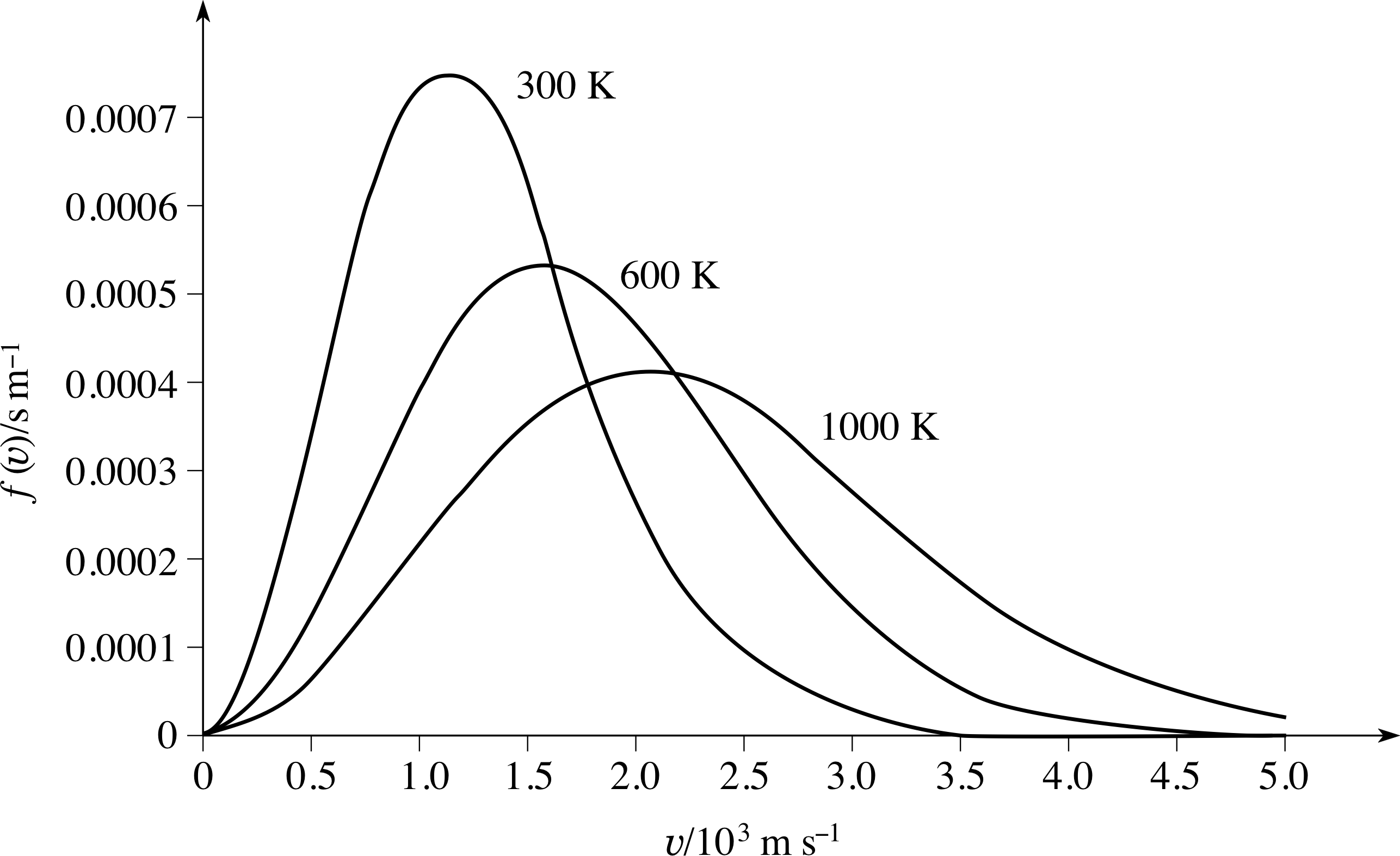
Figure 6 The Maxwell–Boltzmann speed distribution function for a sample of gas at three different temperatures. At higher temperatures, the peak in the distribution function becomes lower, broader, and occurs at a higher speed.
The result of combining the low and high speed behaviours of Equation 30 is that there must be a maximum in the function at some speed, between the quadratic growth regime and the exponential decay regime.
This is illustrated in Figure 6, which shows the shape of the Maxwell–Boltzmann speed distribution function f (υ) for a sample of gas at three different temperatures. The important points to notice here are that as the temperature increases the peak in the distribution becomes lower and broader, and occurs at higher speeds.
The interpretation of f (υ)∆υ as a probability has an important implication for any graph of f (υ) against υ, including the graphs in Figure 6:
The area enclosed between any graph of f (υ) and the υ-axis must be exactly 1 i
(in the scale units appropriate to the graph).
Actually measuring the area under the curves in Figure 6 to verify this would be very time consuming, but you can easily see that it might well be true just by noticing that the 1000 K curve is fairly close to being a triangle with: height 4 × 10⁻⁴ s m−1, base length 5 × 10³ m s−1 and hence area (4 × 10⁻⁴ s m−1 × 5 × 103 m s−1)/2 = 1.
Keeping this constant area requirement in mind will help you to answer Question T11, which concerns the way the distribution function f (υ) changes shape as the temperature parameter T is altered.
Question T11
Explain qualitatively why the peak in the Maxwell– Boltzmann speed distribution function (Figure 6) becomes lower, broader, and moves to higher speeds as the temperature increases.
Answer T11
We know that heating the gas adds translational kinetic energy and so molecular speeds, on average, must increase – so the peak must shift to a higher speed. We also know that the effect of increasing T is to reduce the quantity A (T) and to reduce the exponentially decaying factor in
$f(\upsilon)\Delta\upsilon = 4\pi\left(\dfrac{m}{2\pi kT}\right)^{3/2}\upsilon^2\exp(-m\upsilon^2/2kT)\Delta\upsilon = A(T)\upsilon^2\exp(-m\upsilon^2/2kT)$
The curve for the higher temperature must rise less rapidly at low speeds (as A (T) is less) and fall less rapidly at high speeds (as the exponential factor is less negative).
This implies that the curve is broadened, i.e. there are a wider range of speeds. The area under the whole curve is unity (as the probability for a molecule to have a speed somewhere within the full range is unity). So if the area under the curve stays constant but it is broadened it follows that the curve must reach a lower peak.
Knowing the Maxwell–Boltzmann distribution function we can answer a variety of questions about an ideal gas. For example, there are at least three characteristic speeds that are likely to be of interest:
- 1
-
First, and most obviously, we would like to know the speed corresponding to the peak in the distribution – the most common speed. For obvious reasons we will call this the most probable speed υprob.
- 2
-
Second, we would like to know the average speed $\langle\upsilon\rangle$.
- 3
-
Finally, because of its significance in the kinetic theory link with the ideal gas law, as shown in Subsection 2.4, we would like to know the root-mean-squared speed υrms. This would also allow us to calculate the average kinetic energy per molecule mυrms2/2.
All of these characteristic speeds i can be calculated from the form of the distribution function implied by (Equation 30),
$f(\upsilon)\Delta\upsilon = 4\pi\left(\dfrac{m}{2\pi kT}\right)^{3/2}\upsilon^2\exp(-m\upsilon^2/2kT)\Delta\upsilon$(Eqn 30)
using calculus.
Aside: The most probable speed comes at the peak of the distribution, which can be found from the point at which the gradient of the function becomes zero; using calculus, we find that this corresponds to the speed at which df (υ)/dυ = 0. We must differentiate f (υ) with respect to υ, and set the result equal to zero, and solve the resulting equation to find the appropriate speed υ = υprob. The average speed $\langle\upsilon\rangle$ is given by the integral
$\displaystyle \langle\upsilon\rangle = \int_0^\infty\upsilon f(\upsilon)\,d\upsilon$
and the root-mean-squared speed vrms may be obtained from
$\displaystyle \upsilon_{\rm rms}^2 = \int_0^\infty\upsilon^2 f(\upsilon)\,d\upsilon$
We will not present the mathematical details of these calculations for the three characteristic speeds, but the results are as follows:
the most probable speed$\upsilon_{\rm prob} = \sqrt{\dfrac{2kT}{m}}$(32)
the average speed$\langle\upsilon\rangle = \sqrt{\dfrac{8kT}{\pi m}}$(33)
the root-mean-squared speed$\upsilon_{\rm rms} = \sqrt{\dfrac{3kT}{m}}$(Eqn 12)
We have already derived the expression for υrms in Subsection 2.5, on the basis of a comparison with the ideal gas law; it is reassuring that this result is also derivable from the Maxwell–Boltzmann speed distribution.
Also, Equation 12 confirms that the average kinetic energy per molecule (½ mυ2) is 3kT/2, in agreement with Equation 10,
$\langle\varepsilon_{\rm tran}\rangle = \frac32kT$(Eqn 10)
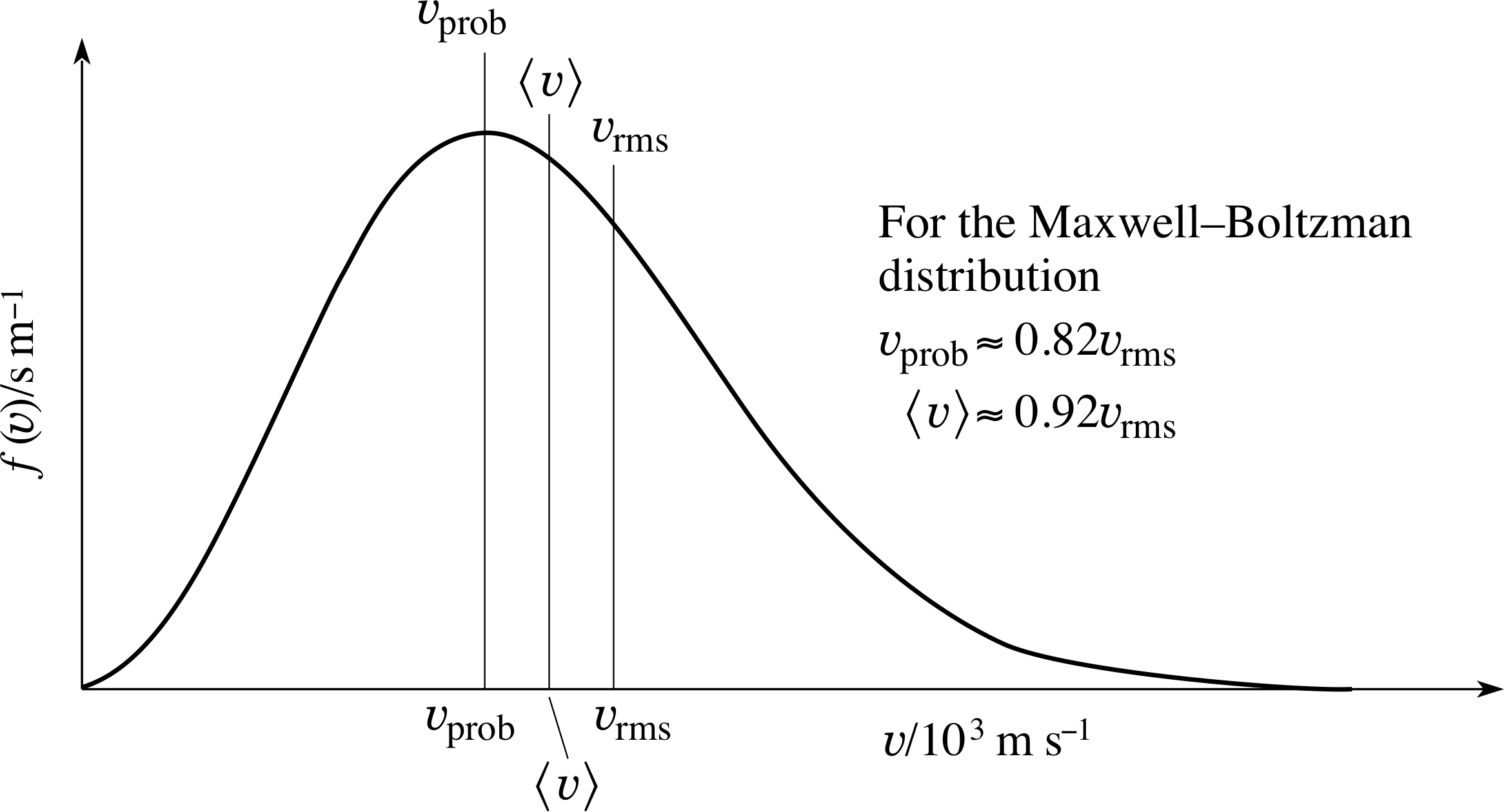
Figure 7 The relationship between υprob, $\langle\upsilon\rangle$ and υrms for the Maxwell–Boltzmann speed distribution.
All three characteristic speeds are proportional to (T/m)1/2, but it is apparent from the numerical factors involved that υrms > $\langle\upsilon\rangle$ > υprob.
Figure 7 shows the relationship between υprob, $\langle\upsilon\rangle$ and υrms for the Maxwell–Boltzmann speed distribution.
For any distribution (where there is a spread of speeds) it is generally true that υrms > $\langle\upsilon\rangle$, but the special results shown in Figure 7 and given by Equations 32, 33 and 12 are specific to the Maxwell–Boltzmann speed distribution. These inequalities lead to the interesting point that, for any distribution, the molecule with the average speed is not the molecule with the average kinetic energy!
Question T12
Suppose we have a very simple speed distribution involving only five molecules. In arbitrary units i their speeds are 1, 2, 2, 3 and 4.
Calculate the three characteristic speeds for this distribution (not Maxwell–Boltzmann) and show that υrms > $\langle\upsilon\rangle$ > υprob.
Explain why υrms > $\langle\upsilon\rangle$ is likely to be true for any distribution.
Answer T12
The average speed for the five molecules is:
$\upsilon = \dfrac{\upsilon_1 + \upsilon_2 + \upsilon_3 + \upsilon_4 + \upsilon_5}{5} = \dfrac{1 + 2 + 2 + 3 + 4}{5} = \dfrac{12}{5} = 2.40$ (in the arbitrary units of the question)
For this very simple distribution the most probable speed, υprob, is 2.
The root-mean-squared (rms) speed is given by Equation 6,
$\upsilon_{\rm rms} = \sqrt{\langle\upsilon^2\rangle}$(Eqn 6)
where
$\langle\upsilon^2\rangle = \dfrac{\upsilon_1^2 + \upsilon_2^2 + \upsilon_3^2 + \upsilon_4^2 + \upsilon_5^2}{5} = \dfrac{1^2 + 2^2 + 2^2 + 3^2 + 4^2}{5} = \dfrac{34}{5} = 6.80$
We find $\upsilon_{\rm rms} = \sqrt{6.80\os} = 2.61$, which confirms the claim, υrms > $\langle\upsilon\rangle$ > υprob.
It can be seen from the averaging processes above that the evaluation of υrms gives additional weight to the higher values of υ as compared to the lower values of υ (by squaring the numbers); in contrast, the calculation of $\langle\upsilon\rangle$ treats large and small speeds equally. It follows that υrms > $\langle\upsilon\rangle$ is true for any distribution (unless all molecules have the same speed).
Question T13
Calculate υprob, $\langle\upsilon\rangle$ and υrms for helium at a temperature of 300 K. The mass of a helium atom is 6.65 × 10⁻²⁷ kg. i
Answer T13
We use Equations 32, 33 and 12,
the most probable speed$\upsilon_{\rm prob} = \sqrt{\dfrac{2kT}{m}}$(32)
the average speed$\langle\upsilon\rangle = \sqrt{\dfrac{8kT}{\pi m}}$(33)
the root-mean-squared speed$\upsilon_{\rm rms} = \sqrt{\dfrac{3kT}{m}}$(Eqn 12)
with the helium mass substituted:
$\upsilon_{\rm prob} = \sqrt{\dfrac{2kT}{m}} = \rm \sqrt{\dfrac{2\times1.38\times10^{-23}\,J\,K^{-1}\times300\,K}{6.65\times10^{-27}\,kg}} = 1.12\,km\,s^{-1}$
$\langle\upsilon\rangle = \sqrt{\dfrac{8kT}{\pi m}} = \rm \sqrt{\dfrac{8\times1.38\times10^{-23}\,J\,K^{-1}\times300\,K}{\pi\times6.65\times10^{-27}\,kg}} = 1.26\,km\,s^{-1}$
$\upsilon_{\rm rms} = \sqrt{\dfrac{3kT}{m}} = \rm \sqrt{\dfrac{3\times1.38\times10^{-23}\,J\,K^{-1}\times300\,K}{6.65\times10^{-27}\,kg}} = 1.37\,km\,s^{-1}$
3.2 The distribution of molecular kinetic energies
We can use the Maxwell–Boltzmann speed distribution to determine how the kinetic energies of the molecules are distributed around the mean kinetic energy, 3kT/2. A molecule with speed υ has translational kinetic energy εtran = mυ2/2. The number of molecules, n (υ)∆υ, having speeds within a narrow range between υ and (υ + ∆υ) will also have translational kinetic energies in the range εtran to (εtran + ∆εtran); we will call this number nε(εtran)∆εtran. The numbers in this speed interval and this energy interval are clearly equal, since they are the same molecules.
Therefore we can write
n (υ)∆υ = nε(εtran)∆εtran
Using Equation 29,
$n(\upsilon)\Delta\upsilon = 4\pi N\left(\dfrac{m}{2\pi kT}\right)^{3/2}\upsilon^2\exp(-m\upsilon^2/2kT)\Delta\upsilon$(Eqn 29)
and substituting εtran = mυ2/2 we have
$n(\upsilon)\Delta\upsilon = 4\pi N\left(\dfrac{m}{2\pi kT}\right)^{3/2}\left(\dfrac{2\varepsilon_{\rm tran}}{m}\right)\exp(-\varepsilon_{\rm tran}/kT)\Delta\upsilon = n_\varepsilon(\varepsilon_{\rm tran})\Delta\varepsilon_{\rm tran}$
or$n_\varepsilon(\upsilon)\Delta\upsilon\left(\dfrac{\Delta\varepsilon_{\rm tran}}{\Delta\upsilon}\right) = 4\pi N\left(\dfrac{m}{2\pi kT}\right)^{3/2}\left(\dfrac{2\varepsilon_{\rm tran}}{m}\right)\exp(-\varepsilon_{\rm tran}/kT)\Delta\upsilon = n_\varepsilon(\varepsilon_{\rm tran})\Delta\varepsilon_{\rm tran}$
Finding an explicit formula for nε(εtran) in terms of εtran (similar to the expression for n (υ) in terms of υ implied by Equation 30),
$f(\upsilon)\Delta\upsilon = 4\pi\left(\dfrac{m}{2\pi kT}\right)^{3/2}\upsilon^2\exp(-m\upsilon^2/2kT)\Delta\upsilon$(Eqn 30)
requires that we express (∆εtran/∆υ) in terms of εtran. This is done by noting that
$\Delta\varepsilon_{\rm tran} = \frac12m(\upsilon + \Delta\upsilon)2 - \frac12m\upsilon^2 = \frac12m\upsilon^2 + m\upsilon\Delta\upsilon + \frac12 m(\Delta\upsilon)^2 - \frac12m\upsilon^2 = m\upsilon(\Delta\upsilon) + \frac12 m(\Delta\upsilon)^2$
But, since the speed range is narrow, ∆υ is small and the term involving (∆υ)2 can be ignored.
Thus ∆εtran ≈ mυ∆υ and so $\dfrac{\Delta\varepsilon_{\rm tran}}{\Delta\upsilon} \approx m\upsilon = \sqrt{2m\varepsilon_{\rm tran}\os}$ i
We therefore have
$n_\varepsilon(\varepsilon_{\rm tran}) = 4\pi N\left(\dfrac{m}{2\pi kT}\right)^{3/2}\left(\dfrac{2\varepsilon_{\rm tran}}{m}\right)\left(\dfrac{1}{2m\varepsilon_{\rm tran}}\right)^{1/2}\exp(-\varepsilon_{\rm tran}/kT)$
i.e.$n_\varepsilon(\varepsilon_{\rm tran}) = 2\pi N\left(\dfrac{1}{\pi kT}\right)^{3/2}\varepsilon_{\rm tran}^{1/2}\exp(-\varepsilon_{\rm tran}/kT)$(34)
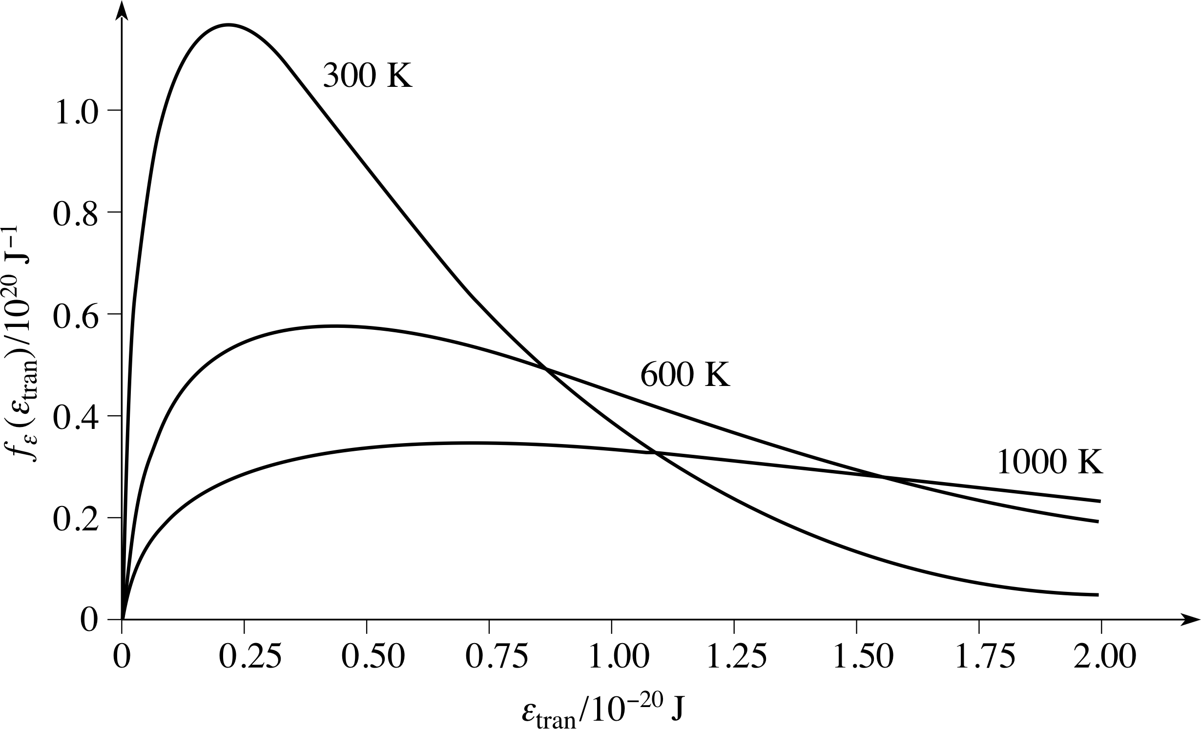
Figure 8 The distribution of molecular kinetic energies associated with the speed distribution. The Maxwell–Boltzmann energy distribution function for a sample of gas at the same three temperatures used for the speed distributions shown in Figure 6.
for the distribution of molecular translational kinetic energy. As before, we can use our knowledge of nε(εtran) to write down a maxwell_boltzmann_energy_distributionMaxwell–Boltzmann energy distribution function, fε(εtran) = nε(εtran)/N, such that fε(εtran)∆εtran is the probability that a molecule chosen at random will have energy in the narrow range εtran to εtran + ∆εtran.
Figure 8 shows the energy distribution function for the same three temperatures used for the speed distributions shown in Figure 6.
It is interesting to note (from Equation 34) that the energy distribution is determined only by the temperature and is independent of the molecular mass; this extends the observation we made in Subsection 2.4, that the average molecular kinetic energy is determined only by the temperature and is independent of the molecular mass. This is in contrast to the average speeds and the distributions over speed which are dependent on the molecular masses, as expected from Subsection 2.5.
3.3 Applications and verification of the speed distribution
In Section 2 we were able to relate the microscopic molecular behaviour of a gas to its macroscopic properties of pressure and temperature. This relationship did not involve any particular speed distribution but only required there to be an average molecular translational kinetic energy. In contrast, there are other properties of gases which do depend on the details of the speed distribution. Examples of such properties are:
- 1
-
The inter–mixing of gases (same or different) when there are local differences of concentrations present; this process is called diffusion.
- 2
-
Viscosity or gas friction, in which layers of gas in relative motion tend to inter–mix and thereby reduce the relative motion.
- 3
-
Thermal conduction, when there are temperature gradients present in a gas, in which inter–mixing of gas from the hot and cold regions tends to equalize the average speeds and hence the temperatures in each region.
You will realize that these three properties are related in that they are each controlled by the rate of molecular inter-mixing, or how quickly molecules can find their way from one region to another region of the gas. This rate will be limited due to intermolecular collisions, which slow down the rate of transport. It is perhaps not surprising then that these three properties are collectively known as transport processes. These transport processes can each be predicted assuming the speed distribution and the agreement between the predicted and measured properties then gives strong indirect support for the validity of the Maxwell–Boltzmann speed distribution itself. i
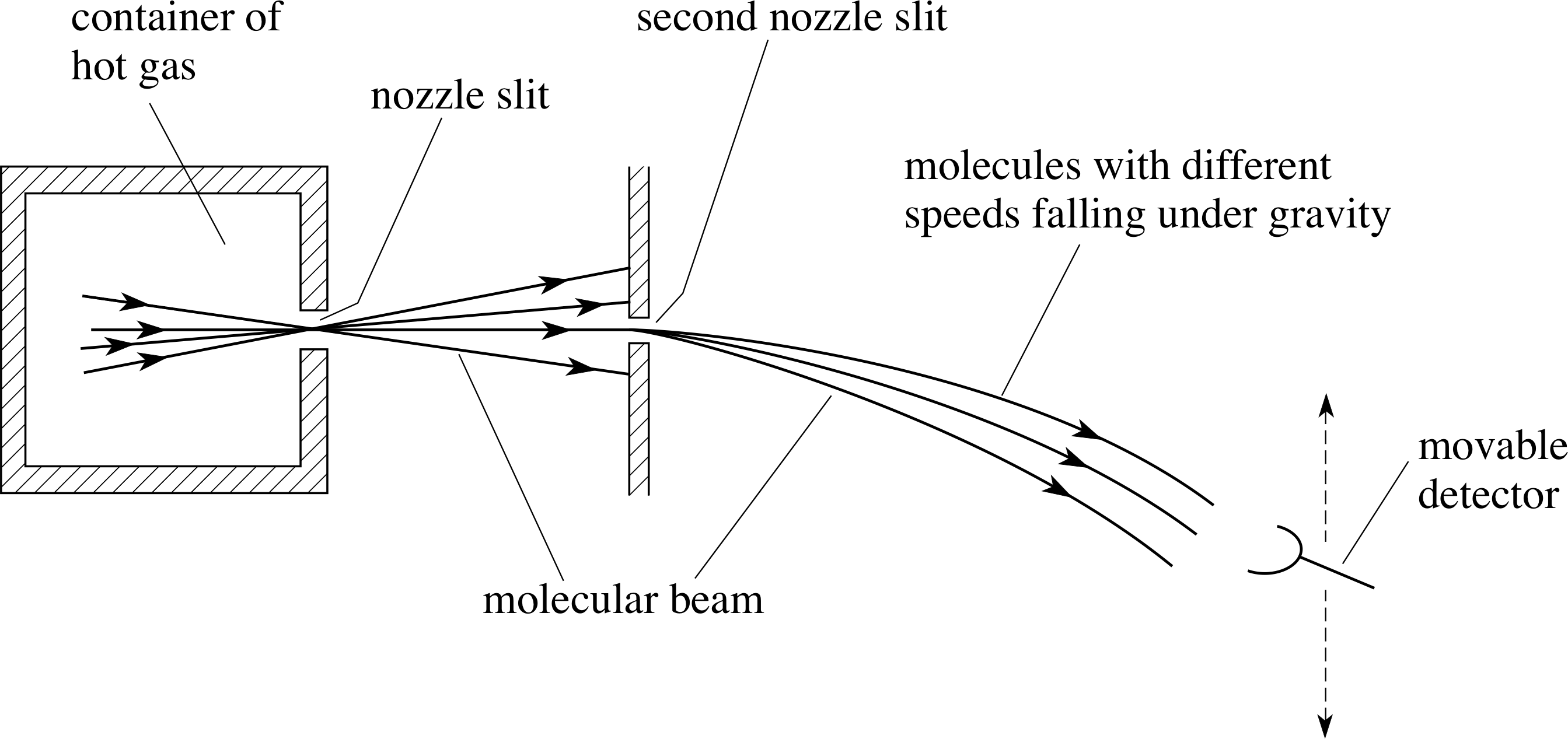
Figure 9 A method of measuring molecular speeds that can be used to demonstrate the Maxwell–Boltzmann speed distribution. The whole apparatus is enclosed in a sealed evacuated chamber.
The validity of the Maxwell–Boltzmann speed distribution can also be demonstrated from direct measurement of the distribution of molecular speeds in a gas. How can we accomplish this? We cannot measure the speed of individual molecules, so we need to make some measurement that directly depends on their speeds. One method of performing such measurements is shown in Figure 9. We generally begin by taking a container of gas and place a fine slit in the side (termed a nozzle). When molecules from inside strike the slit space they emerge from the slit. If the region beyond the slit is a good vacuum these emerging molecules continue on in the same direction.
If we then interpose a second fine slit some distance downstream we will select only those molecules travelling in a particular direction. Such a beam, with a well–defined direction, is called a molecular beam.
Molecules in such a molecular beam, when launched horizontally, will tend to fall due to gravity and if the vertical drop to a distant detector is measured this can be related to the time of flight and hence to the molecular speed. Careful interpretation i of the numbers of molecules arriving as a function of the distance dropped confirms the form of the speed distribution, but the details of the method need not concern us here.
3.4 Summary of Section 3
The Maxwell–Boltzmann speed distribution for a gas has been introduced but not derived. This distribution gives the numbers of molecules within a narrow speed range as a function of the speed. From this expression it is possible to identify three characteristic speeds for a gas: these are the most probable speed, the average speed and the root-mean-squared speed – arranged in order of increasing magnitude. The distribution of molecular kinetic energies associated with the Maxwell–Boltzmann speed distribution has been derived from the speed distribution and this is seen to be independent of the molecular mass, being determined only by the temperature. Finally, both indirect and direct evidence in support of the Maxwell–Boltzmann speed distribution has been given in terms of transport processes and the speeds in molecular beams, respectively.
4 A more realistic model of a gas
4.1 Van der Waals equation of state
It was discovered through careful measurements in the 19th century that the ideal gas equation of state was only an approximation to the true behaviour of real gases. The Dutch physicist Johannes van der Waals (1837–1923) devised the following generalization to the ideal gas equation of state in order to describe more accurately the behaviour of real gases:
$\left(P + \dfrac{a}{V_{\rm m}^2}\right)(V_{\rm m}-b) = RT$(35)
This is known as van der Waals equation of state.
| a/10−1 m6 Pa mol−2 | b/10−5 m3 mol−1 | |
|---|---|---|
| nitrogen (N2) | 0.035 | 2.4 |
| oxygen (O2) | 1.41 | 3.91 |
| xenon (Xe) | 1.38 | 3.18 |
| helium (He) | 4.25 | 5.10 |
In this equation, Vm represents the volume per mole; a and b can be regarded as empirical constants, although they have a theoretical interpretation in terms of a kinetic theory model.
The values of a and b vary from one gas to another, as indicated in Table 1. We want to consider briefly what the physical origin of such terms might be in terms of our kinetic theory model of a gas.
Question T14
What should be the dimensions of a and b in order that Equation 35 should be dimensionally consistent? Are the units in Table 1 appropriate?
Answer T14
To be dimensionally consistent, the terms within any set of brackets must have the same units.
Thus, the units of b must be m3 mol−1 and a/Vm must be in Pa (= N m−2).
So a must have the units of P × Vm2 and since Vm has units of m6 mol−2, this means that the units of a are N m−2 × m6 mol−2, or N m4 mol−2. Therefore the units given in Table 1 are correct.
4.2 Excluded volumes
In Subsection 2.4, in deriving the ideal gas equation of state, we ignored the volume taken up by the gas molecules themselves. Although reasonable, this approximation has repercussions. For example, the ideal gas equation of state implies that the volume of the gas approaches zero when the temperature approaches zero, whereas in reality the minimum volume that the gas can occupy must exceed the total molecular volume.
If we consider the molecules to be perfect spheres of radius r, then on touching, the molecules will be separated by 2r. This means that the centre of a second molecule will be excluded from a sphere of radius 2r, whose volume equals $\frac43\pi(2r)^3$, which is eight times the individual molecular volume. Thus the excluded volume per molecule for spheres is four times the molecular volume.
For one mole of gas, the total volume excluded by the finite size of the molecules will be NA × 4 × υm, where υm is the individual molecular volume. We might then predict that the appropriate generalization for the ideal gas would be to replace the volume per mole, V/n, by (Vm − 4υmNA). This identifies the constant b in the van der Waals equation of state with 4υmNA:
$\left(P + \dfrac{a}{V_{\rm m}^2}\right)(V_{\rm m}-b) = RT$(Eqn 35)
4.3 Intermolecular forces
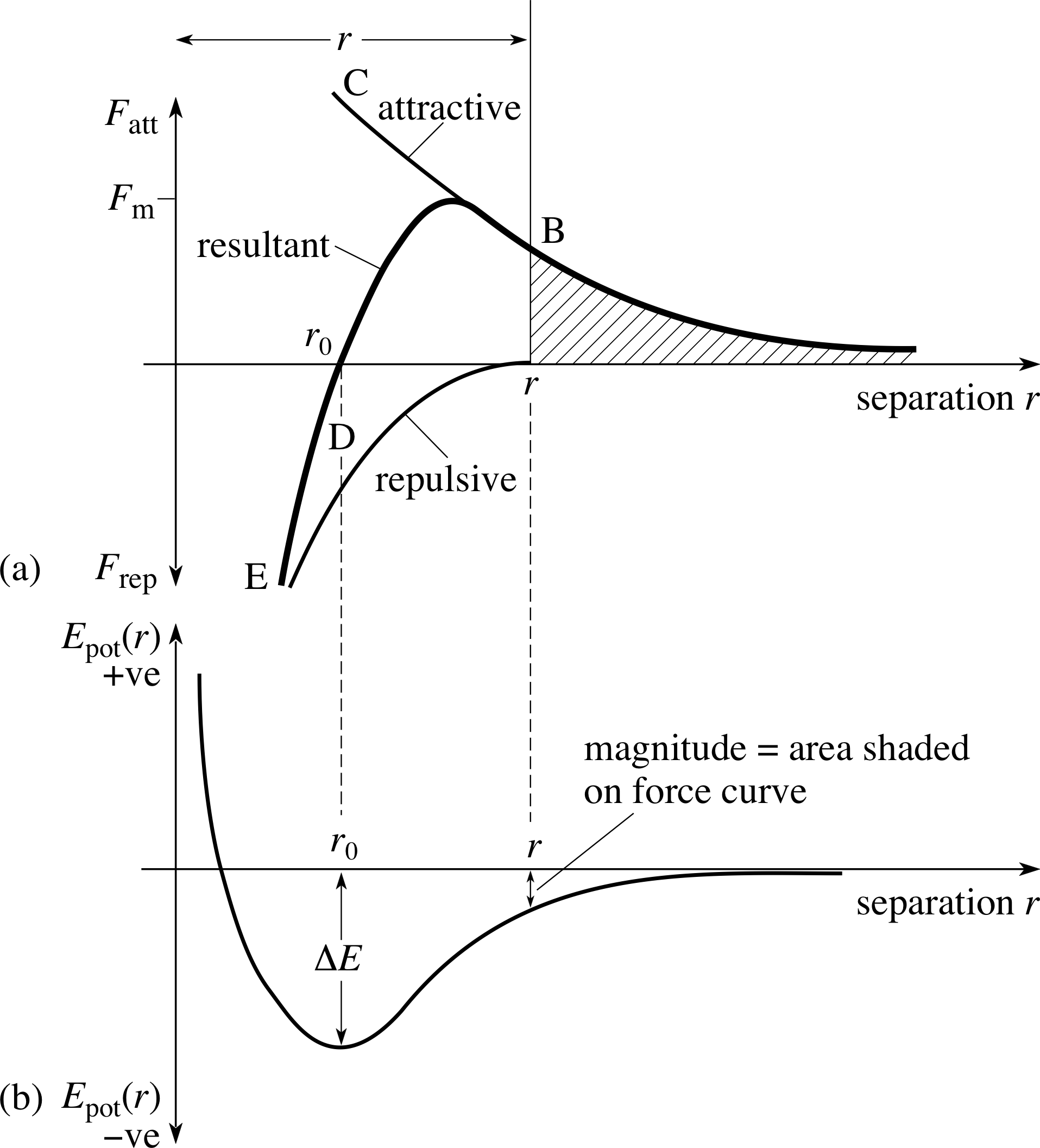
Figure 10 Typical variation of (a) the intermolecular force and (b) the corresponding potential energy for two molecules separated by a distance r. When the molecules are very close together there is a repulsive force (as at point E), when they are far apart the force is attractive (as at B).
We now test our assumption that the long–range forces between molecules are negligible. Figure 10 shows a typical variation in (a) intermolecular force, and (b) the corresponding potential energy curves for the interaction between two molecules.
Figure 10a shows that there is a large repulsive force between molecules when they are very close to each other, and a relatively weak attractive force at larger separations. i
This is to be expected, since we know that most gases will condense to form a liquid if we cool them enough, and this would only happen if there were an attractive force that pulled the molecules together (this was actually van der Waals motivation in deriving his equation). The short–range strong repulsion accounts for the collisional forces and the success of the hard sphere model. What effect will the weak long–range attractive force have on the ideal gas equation of state? Let us consider a single reference molecule as it moves towards a wall.
In the centre of the volume of gas, there will be (on average) an equal number of gas molecules on all sides of our reference molecule, so that the net force will be approximately zero. When our reference molecule approaches a wall of the container, there will be more gas molecules on the side away from the wall than on the side toward the wall, and ultimately (just before the collision with the wall) all other gas molecules will be on the side away from the wall. The reference molecule will then feel a weak attraction from the remaining molecules in the gas, which will tend to reduce its velocity before impact with the wall and hence reduce the change in momentum on colliding with the wall. This will reduce the effective pressure compared with the gas at the same temperature but without such attractive forces.
What form will this reduction take? The reduction in pressure must depend on the size of the attractive force on each molecular impact and on the number of these impacts per second. The force depends on the number of molecules in the gas which are within range, and for a fixed number of molecules (e.g. per mole) this will depend inversely on the volume. Also, for a fixed number of molecules, the rate of molecular impacts depends on the pressure – which also will depend inversely on the volume. These two multiplying factors, each proportional to 1/Vm, suggest that the effective pressure reduction should be proportional to 1/Vm2. Since we have not evaluated any actual forces, we can only say that the pressure should be less by some term proportional to 1/Vm2. This effect is reproduced by replacing the term P in the ideal gas equation of state by a term (P + a/Vm2), as in the van der Waals equation of state, to restore the effective pressure reduction.
$\left(P + \dfrac{a}{V_{\rm m}^2}\right)(V_{\rm m}-b) = RT$(Eqn 35)
Question T15 i
If there is an appreciable attractive force between the molecules of the gas, there should be a similar attractive force between the gas molecules and the molecules of the containing walls. Consider the effect of this additional force on the molecular encounters with the wall and argue what effect this will have on the pressure exerted on the walls by the gas.
Answer T15
Perhaps surprisingly, the answer is that there is no effect at all – whatever the details of the force!
For simplicity, consider an attractive force which comes into play only very near the wall. This force will accelerate the molecules into the collision but decelerate them after the collision. The net change of momentum of the molecules will be the same as in the ‘no force’ situation and it will be as if no force were operating.
5 Closing items
5.1 Module summary
- 1
-
The macroscopic or bulk properties of an ideal gas, as given by the ideal gas law
PV = nRT(Eqn 1)
can be derived from a simple microscopic model of the behaviour of molecules within the gas, based on certain fundamental assumptions. This model is known as the kinetic theory.
- 2
-
The kinetic theory calculation of the pressure due to an ideal gas leads to a form of the equation of state which allows us to associate the average translational kinetic energy per molecule with the absolute temperature. This enables us to give a microscopic interpretation to the macroscopic concept of temperature.
$PV = \frac23N\langle\varepsilon_{\rm tran}\rangle$(Eqn 7)
$\langle\varepsilon_{\rm tran}\rangle = \frac32kT$(Eqn 10)
where$k = \dfrac{nR}{N} = \dfrac{R}{N_A}$ is Boltzmann’s constant.
- 3
-
The kinetic theory can also be used to give microscopic interpretations of the internal energy and specific heats of gases, in terms of the number of molecular degrees of freedom q and the equipartition of energy theorem:
$E_{\rm int} = \dfrac q2NkT$(Eqn 15)
$C_V = \dfrac q2R\quad\text{and}\quad C_P = \left(1 + \dfrac q2\right)R$(Eqns 18 and 24)
$C_P - C_V= R\quad\text{and}\quad\gamma = \dfrac{C_P}{C_V} = 1 + \dfrac2q$(Eqns 22 and 23)
- 4
-
The mean free path is the average distance travelled by molecules between collisions. The mean free time is the average time between collisions. A value for these, given specified conditions, can also be calculated from kinetic theory.
- 5
-
The random nature of molecular motion leads to an expression for the distribution of speeds among the gas molecules; this is the Maxwell–Boltzmann speed distribution:
$f(\upsilon) = 4\pi\left(\dfrac{m}{2\pi kT}\right)^{3/2}\upsilon^2\exp(-m\upsilon^2/kT)$
The distribution can be characterized in terms of a most probable speed, an average speed and a root-mean-squared speed. The Maxwell–Boltzmann speed distribution has been verified experimentally, indirectly through its effect on transport processes and directly by measuring molecular speeds in a molecular beam.
- 6
-
The van der Waals equation of state,
$\left(P + \dfrac{a}{V_{\rm m}^2}\right)(V_{\rm m}-b) = RT$(Eqn 35)
provides a more accurate description of real gases than the ideal gas equation. Its empirically determined parameters can be explained in terms of modifications to the simple kinetic theory, through excluded volumes and intermolecular forces.
5.2 Achievements
Having completed this module, you should be able to:
- A1
-
Define the terms that are emboldened and flagged in the margins of the module.
- A2
-
Describe and explain the basic assumptions underpinning the kinetic theory of gases.
- A3
-
Explain qualitatively how the kinetic theory model of a gas is in accord with the ideal gas equation of state PV = nRT.
- A4
-
Make approximate calculations of mean free paths and mean free times, given appropriate molecular data.
- A5
-
Carry out simple calculations based on the kinetic theory equation,
$PV = \frac23N\langle\varepsilon_{\rm tran}\rangle$(Eqn 7)
- A6
-
Recall and explain the significance of the equation
$\langle\varepsilon_{\rm tran}\rangle = \frac32kT$(Eqn 10)
and use it in calculations.
- A7
-
Explain the interpretation of the internal energy of a gas in terms of the kinetic theory model and calculate internal energies and specific heats in terms of degrees of freedom for different types of molecules.
- A8
-
Recall the equation relating υrms to absolute temperature and molecular mass and be able to use it in calculations.
- A9
-
Explain what is meant by the Maxwell–Boltzmann speed distribution, sketch its form and briefly explain how it may be tested.
- A10
-
Distinguish between the quantities υprob, $\langle\upsilon\rangle$ and υrms for the Maxwell–Boltzmann speed distribution and explain why they differ and how their magnitudes compare (without detailed formulae).
- A11
-
Describe the physical reasoning behind the modifications to the ideal gas equation of state which lead to the van der Waals equation of state.
- A12
-
Use the van der Waals equation of state to calculate physical parameters.
Study comment You may now wish to take the following Exit test for this module which tests these Achievements. If you prefer to study the module further before taking this test then return to the topModule contents to review some of the topics.
5.3 Exit test
Study comment Having completed this module, you should be able to answer the following questions each of which tests one or more of the Achievements.
You may need to use the following values in the Exit test questions:
NA = 6.02 × 10²³ mol−1 R = 8.314 J K−1 mol−1 k = 1.381 × 10⁻²³ J K−1
Question E1 (A2 and A3)
Summarize the key assumptions of the kinetic theory of ideal gases. Explain how the concept of randomness is crucial to the theory.
Answer E1
The key assumptions of the kinetic theory of ideal gases are:
- 1
-
The ideal gas consists of a large number of identical molecules in random motion.
- 2
-
All collisions, whether between molecule and molecule, or between molecule and wall, are elastic.
- 3
-
The individual molecules and collisions obey Newton’s laws of motion.
- 4
-
The molecules experience only contact forces. They interact only when actually touching, like hard spheres.
- 5
-
The volume occupied by the molecules themselves is negligible compared to the volume occupied by the gas as a whole.
The concept of randomness is important because it allows us to avoid dealing with the individual microscopic collisions, and furthermore assures us that the details of such individual collisions are irrelevant, because they are averaged out by the overall random nature of the system.
(Reread Subsections 2.1 and 2.2 if you had difficulty with this question.)
Question E2 (A4)
The mass density of helium gas at a temperature of 273 K and a pressure of 1.01 × 10⁵ Pa is 0.178 kg m−3 and the mean free path is found to be 285 nm. The mass of one mole of helium is 4.00 g.
Using the kinetic theory model:
(a) What is the number density for helium under these conditions?
(b) What is the effective atomic diameter?
Answer E2
(a) The number density (denoted by nρ) can be calculated by taking the ratio of the mass density to the mass per molecule:
so$n_\rho = \dfrac{\rho}{m} = \dfrac{\rho}{\text{(mass of 1 mole of gas / Avogadro’s number)}} = \rm \dfrac{0.178\,kg\,m^{-3}}{(4.00\times10^{-3}\,kg/6.02\times10^{23})} = 2.68\times10^{25}\,m^{-3}$
(b) We need to use the equation for the mean free path,
$\lambda = \dfrac{1}{4\sqrt{2\os}\pi r^2n_\rho}$(Eqn 28)
which we can rearrange to solve for the radius r:
$r = \left(\dfrac{1}{4\sqrt{2\os}\pi r^2n_\rho}\right)^{1/2} = \rm \left(\dfrac{1}{4\sqrt{2\os}\pi\times2.68\times10^{25}\,m^{-3}\times285\times10^{-9}\,m}\right)^{1/2}$
$r = \rm \left(\dfrac{1}{1.36\times10^{20}\,m^{-2}}\right)^{1/2} = (7.37\times10^{-21}m^2)^{1/2} = 8.58\times10^{-11}\,m = 0.0858\,nm$
So the atomic diameter = 2r = 0.172 nm.
(Reread Subsection 2.8 if you had difficulty with this question.)
Question E3 (A5 and A6)
Fifteen moles of a monatomic ideal gas are at a pressure of 1.8 × 10⁵ Pa in a container of volume 0.25 m3.
(a) What is the temperature of the gas
(b) What is the average kinetic energy of a gas molecule?
Answer E3
(a) Using the ideal gas equation of state, we find
$T = \dfrac{PV}{nR} = \rm \dfrac{1.8\times10^5Pa\times0.25\,m^3}{15\,mol\times8.314\,J\,K^{-1}\,mol^{-1}} = 361\,K$
(b) The average molecular translational kinetic energy is given by
$\varepsilon_{\rm tran} = \dfrac32kT = \rm 1.5\times1.381\times10^{-23}\,J\,K^{-1}\times361\,K = 7.48\times10^{-21}\,J$
(Reread Subsections 2.1 and 2.5 if you had difficulty with this question.)
Question E4 (A7)
2.0 moles of a monatomic ideal gas and 2.0 moles of a diatomic ideal gas (with no vibrational degrees of freedom) are at a common temperature of 300 K. What are the total internal energies of the two gases?
Answer E4
The internal energy of a monatomic gas is given by $\frac32NkT = \frac32nRT$.
For a diatomic molecule (with no vibrational motion) it is $\frac52NkT = \frac52nRT$.
Thus:
$(E_{\rm int})_{\rm monatomic} = \frac32\times nRT = \rm 1.5\times2.0\,mol\times8.314\,J\,K^{-1}mol^{-1}\times300\,K = 7.5\,kJ$
$(E_{\rm int})_{\rm diatomic} = \frac52\times nRT = \rm 2.5\times2.0\,mol\times8.314\,J\,K^{-1}mol^{-1}\times300\,K = 12.5\,kJ$
(Reread Subsection 2.6 if you had difficulty with this question.)
Question E5 (A7 and A8)
Normal dry air is composed (by volume) mainly of N2 (78.08%), O2 (20.94%), and Ar (0.93%), with a variety of other constituents making up the remaining 0.05%. The mass of one mole of each of these gases is 28.01 g, 32.00 g and 39.95 g, respectively.
(a) At a temperature of 295 K, what are the root-mean-squared speeds of the three main constituents of dry air?
(b) Dry air has a specific heat at constant volume of approximately 20.5 J mol−1 K−1. If the specific heat of a mixture of gases can be taken as the sum of the specific heats due to each gas, is this consistent with air as a mixture of ideal gases, as above?
Answer E5
(a) The rms speed is given by Equation 12,
$\upsilon_{\rm rms} = \sqrt{\dfrac{3kT}{m}} = \sqrt{\dfrac{3RT}{N_Am}}$ (since R = NAk)
where NAm represents the mass per mole of the gas in question. So for nitrogen:
$\upsilon_{\rm rms}(\rm N_2) = \rm \sqrt{\dfrac{3\times8.314\,J\,K^{-1}\,mol^{-1}\times295\,K}{28.01\times10^{-3}\,kg\,mol^{-1}}} = \sqrt{2.63\times10^5\,m^2\,s^{-2}} = 513\,m\,s^{-1}$
Similar calculations for the other two gases give:
υrms (O2) = 480 m s−1 and υrms (Ar) = 429 m s−1
(b) We can calculate the specific heat at constant volume for a mixture of gases by taking the weighted average of the individual specific heats, where the weighting is the fractional composition of the gas.
For dry air as given, we would then have:
CV ≈ 0.7808 × CV (N2) + 0.2094 × CV (O2) + 0.0093 × CV (Ar)
Now if we assume that the gases are ideal, we know that the molar specific heats at constant volume are $\frac52R$ for diatomic gases (assuming no vibrational motion) and $\frac32R$ for monatomic gases. So we can write:
$C_V \approx (0.7808\times\frac52R) + (0.2094\times\frac52R) + (0.0093\frac32R)$
$\phantom{C_V }\approx \rm (1.952+0.5235+0.0140)\times8.314\,J\,K^{-1}\,mol^{-1} = 20.7\,J\,K^{-1}mol^{-1}$
So the agreement is quite good, being within 1%.
(Reread Subsections 2.5 and 2.7 if you had difficulty with this question.)
Question E6 (A8 and A10)
Nitrogen molecules in a container are found to have a root-mean-squared speed of 521 m s−1 and a molar mass (i.e. mass per mole) of 28.01 × 10⁻³ kg mol−1.
(a) Assuming ideal gas behaviour, what is the temperature of the gas
(b) What are the average and most probable speeds for nitrogen molecules in this gas?
(c) What is the ratio $\left.\langle\upsilon^2\rangle\middle/\langle\upsilon\rangle^2\right.$ for this gas? Will this ratio change if the gas is heated?
Answer E6
(a) We need to rearrange Equation 12,
$\upsilon_{\rm rms} = \sqrt{\dfrac{3kT}{m}}$(Eqn 12)
in terms of T to find:
$T = \dfrac{m\upsilon_{\rm rms}^2}{3k}$
The molar mass Mm = NAm and molar gas constant R = NAk,
so$T = \dfrac{M_{\rm m}\upsilon_{\rm rms}^2}{3R} = \rm \dfrac{28.01\times10^{-3}\,kg\,mol^{-1}\times(521\,m\,s^{-1})^2}{3\times8.314\,J\,K^{-1}\,mol^{-1}} = 305\,K$
so$T = \rm \dfrac{7.603\times10^3\,kg\,m^2\,s^{-2}\,mol^{-1}}{24.94\,J\,K^{-1}\,mol^{-1}} = 305\,K$
(b) From Equations 32, 33 and 12,
the most probable speed$\upsilon_{\rm prob} = \sqrt{\dfrac{2kT}{m}}$(Eqn 32)
the average speed$\langle\upsilon\rangle = \sqrt{\dfrac{8kT}{\pi m}}$(Eqn 33)
the root-mean-squared speed$\upsilon_{\rm rms} = \sqrt{\dfrac{3kT}{m}}$(Eqn 12)
we have:
$\langle\upsilon\rangle = (8/3\pi)^{1/2}\upsilon_{\rm rms}\quad\text{and}\quad\upsilon_{\rm prob} = (2/3)^{1/2}\upsilon_{\rm rms}$
In this case these expressions give:
the average speed $\langle\upsilon\rangle$ = 0.921 × 521 m s−1 = 480 m s−1
and the most probable speed is
υprob = 0.816 × 521 m s−1 = 425 m s−1
(c) Using $\langle\upsilon\rangle = (8/3\pi)^{1/2}\upsilon_{\rm rms}$ we can use Equation 6,
$\upsilon_{\rm rms} = \sqrt{\langle\upsilon^2\rangle}$(Eqn 6)
to write:
$\dfrac{\langle\upsilon^2\rangle}{\langle\upsilon\rangle^2} = \left(\dfrac{\upsilon_{\rm rms}}{\langle\upsilon\rangle}\right)^2 = \dfrac{3\pi}{8} \approx 1.18$
which is clearly independent of temperature or, indeed, the gas identity. As a check of our earlier calculations, we can also calculate 5212/4802 = 1.18.
(Reread Subsection 3.1 if you had difficulty with this question.)
Question E7 (A9)
Briefly describe the sort of experimental evidence which supports the Maxwell–Boltzmann speed distribution.
Answer E7
The Maxwell–Boltzmann speed distribution has been verified experimentally, indirectly through its effect on transport processes (such as diffusion, viscosity and thermal conductivity) and directly by measuring molecular speeds in a molecular beam.
This is discussed more fully in Subsection 3.3.
Study comment This is the final Exit test question. When you have completed the Exit test go back and try the Subsection 1.2Fast track questions if you have not already done so.
If you have completed both the Fast track questions and the Exit test, then you have finished the module and may leave it here.
Study comment Having seen the Fast track questions you may feel that it would be wiser to follow the normal route through the module and to proceed directly to the following Ready to study? section.
Alternatively, you may still be sufficiently comfortable with the material covered by the module to proceed directly to the Section 5Closing items.