PHYS 7.6: Mechanical properties of matter |
PPLATO @ | |||||
PPLATO / FLAP (Flexible Learning Approach To Physics) |
||||||
|
1 Opening items
1.1 Module introduction
In this module we consider the response of matter to external forces, but always under the application of balanced forces so there is no acceleration of the body as a whole. We are interested in the manner in which the external forces distort or deform a body.
In Section 2 we examine solids and the ways of characterizing their behaviour in terms of their elastic properties. We introduce the properties of elasticity and plasticity, stress, strain, Hooke’s law and Young’s modulus. We consider tensile, uni-axial compressive, shear and bulk compressive stresses and strains, introducing shear modulus and bulk modulus. In Section 3 we then examine fluids and describe the more limited, but equally important, ways in which they respond to external forces. This discussion includes hydrostatic pressure, Pascal’s principle, Archimedes’ principle and the phenomenon of buoyancy.
In Section 4 we then consider in some detail the ways in which both solids and liquids interact with their environment through effects which occur at surfaces and interfaces, including the familiar phenomenon of friction between solids and the analogous process of viscosity with fluids. We introduce the usual phenomenological descriptions of these, as well as briefly discussing their microscopic basis. Stoke’s law is described, and the existence of a terminal speed for a body falling through a fluid is discussed. Finally, we describe the phenomena of surface tension and capillarity.
Study comment Having read the introduction you may feel that you are already familiar with the material covered by this module and that you do not need to study it. If so, try the following Fast track questions. If not, proceed directly to the Subsection 1.3Ready to study? section.
1.2 Fast track questions
Study comment Can you answer the following Fast track questions? If you answer the questions successfully you need only glance through the module before looking at the Subsection 5.1Module summary and the Subsection 5.2Achievements. If you are sure that you can meet each of these achievements, try the Subsection 5.3Exit test. If you have difficulty with only one or two of the questions you should follow the guidance given in the answers and read the relevant parts of the module. However, if you have difficulty with more than two of the Exit questions you are strongly advised to study the whole module.
Question F1
An aluminium beam has length 1.00 m, a square cross section of side 2.00 mm, and a Young’s modulus of 7.00 × 10¹⁰ N m−2. If a tensile force of 1.00 × 10³ N is applied along the length of the beam, what will be the change in the length of the beam, assuming Hooke’s law is valid?
Answer F1
The applied tensile stress is
$\sigma_{\rm T} = \rm \dfrac{1.00\times10^3\,N}{(2.00\times10^{-3}\,m)^2} = 2.50\times10^8\,Pa$
Using Hooke’s law, we have:
σT = 2.50 × 10⁸ Pa = YεT
so$\varepsilon_{\rm T} = \dfrac{2.50\times10^8\,Pa}{7.00\times10^{10}\,Pa} = 3.6\times10^{-3}$
Then ∆l = lεT = 3.6 × 10−3 × 1.00 m = 3.6 mm (beam is stretched).
Question F2
Brass has a density of 8.60 × 10³ kg m−3. A small brass weight of mass 10.0 g is dropped into a container of water with density 1.00 × 10³ kg m−3. Taking into account the effect of buoyancy, what would be its apparent weight while submerged in the water?
Answer F2
The apparent weight is given by the difference between the weight and the buoyancy force, which is the weight of fluid displaced. So we have:
Wapp = (ρbrass − ρwater)gV and V = m/ρbrass
and so we can write:
$W_{\rm app} = \left(1-\dfrac{\rho_{\rm water}}{\rho_{\rm brass}}\right)mg = \rm \left(1-\dfrac{1.00\times10^3\,kg\,m^{-3}}{8.60\times10^3\,kg\,m^{-3}}\right)\times10^{-2}\,kg\times9.8\,m\,s^{-2} = 8.67\times10^{-2}\,N$
Question F3
For a bubble the pressure differential across the film is given by 4γ/R, where γ is the surface tension and R is the radius of the bubble. Suppose a soap bubble has γ = 2.50 × 10⁻² N m−1, and is drifting in the air in a room, which has a pressure of 1.0100 × 10⁵ N m−2. If the bubble has a radius of 5.00 mm, what is the pressure inside it?
Answer F3
The difference between the internal and external pressure is given by:
$P-P_{\rm ext} = \dfrac{4\gamma}{R} = \rm \dfrac{4\times2.50\times10^{-2}\,N\,m^{-1}}{5.00\times10^{-3}\,m} = 20.0\,Pa$
so that
P = (1.0100 × 10⁵ Pa) + (0.0002 × 10⁵ Pa) = 1.0102 × 10⁵ Pa
1.3 Ready to study?
Study comment Before beginning the study of this module you should have a clear understanding of the following terms from mechanics: energy, equilibrium, force, normal reaction force, frictional force, gravitational force (weight) mg, centre of gravity, density, and work done by a force. In addition, you should have a qualitative appreciation of the atomic basis of matter and of the existence of interatomic or intermolecular forces at the microscopic level, as well as the concepts of random molecular motion. If you are uncertain of any of these terms you can review them in the Glossary, which will indicate where in FLAP they are developed.
For these questions you may take the magnitude of the acceleration due to gravity to be 9.8 m s−2.
Question R1
An object is in mechanical equilibrium, strung between two vertical cables attached to its top and bottom. The object has a mass of 40.0 kg. If the upper cable exerts a force of 500 N, what is the force exerted by the lower cable?
Answer R1
Since the object is in equilibrium, the sum of the forces must be zero. Since all the forces act along a single line, if T is the tension in the lower cable we have:
0 = 500 N − (40.0 kg × 9.81 m s−2) − T
and soT = 500 N − 392 N = 108 N
(Consult the Glossary for terms about which you are unclear)
Question R2
A wooden block with a mass of 5.00 kg is resting on a horizontal table top. (a) What is the magnitude and direction of the normal reaction force exerted by the table on the block? (b) If a horizontal force of 2.00 N now acts on the block and moves the block a distance of 3.50 m along the surface, calculate the work done by this force and also by the reaction force.
Answer R2
(a) The normal reaction force balances the weight of the block, so it is directed upward from the table and it has a magnitude_of_a_vector_or_vector_quantitymagnitude equal to the weight of the block, so
R = 5.00 kg × 9.81 m s−1 = 49.1 N
(b) The work done W by a force F is the scalar product of the force and the displacement s. This can be found from the product of the magnitude of the force and the displacement in the direction of the force. For the horizontal force this is:
W = F ⋅ s = Fs cos 0° = Fs = 2.00 N × 3.50 m = 7.00 N m = 7.00 J
For the reaction force this is W = R ⋅ s = Rs cos 90° = 0 J.
(Consult the Glossary for terms about which you are unclear)
2 Mechanical properties of solids
2.1 Elasticity: stress, strain, Hooke’s law and Young’s modulus

Figure 1 Forces are applied perpendicular to the two ends of a rod: the net force on the rod is zero because the applied forces have equal magnitudes, but opposite directions.

Figure 2 A model for a solid rod with complicated interatomic forces replaced by springs. External forces are applied only to the end atoms in the rod.
The application of external forces to an object will lead to acceleration if the net force is not zero. In this module we are interested in the application of balanced forces, as indicated in Figure 1, so that the net force will be zero. This topic is part of the study of statics in mechanics.
In such a case, our initial reaction might be to claim that nothing happens, but this overlooks the fact that the rod is not a simple point object. It is a complicated arrangement of atoms and the application of the external forces can affect that arrangement. To make the analysis easier, we assume that the rod is uniform, so that both the composition and cross section are constant over the entire length. We are interested in just how the arrangement of the atoms changes, and we would guess that with forces as shown in Figure 1 (termed tensile forces) the rod would stretch, even if only slightly. At the microscopic level we can visualize this as the atoms being pulled slightly apart. Figure 2 displays a simplified microscopic model for this rod as a row of atoms connected by springs.
The springs are an oversimplified representation of the more complicated interatomic forces present. When we apply the forces to the end of the rod we can visualize the result as each spring being stretched uniformly by an amount that would just result from the forces being applied directly to the individual atom– spring system. We assume that the forces are applied uniformly across the ends of the rod. If we have N atom chains making up the cross section of the rod then the total force will be distributed equally among those N chains. So, we might expect the physics to be determined by the ratio of the force applied to the number of atomic chains. Since we are taking the cross section to be uniform we will have a certain number of chains per unit area (a very large number!). So we will obtain a sensible measure of the effect of the force by taking the perpendicular component of the force F⊥ and by dividing this by the cross–sectional area of the rod. This ratio is given the name stress, and we will denote it by σ (the Greek letter sigma). This particular type of stress, where a body is subject to a stretching force is called a tensile stress, represented as σT.
tensile stress $\sigma_{\rm T}= \dfrac{\text{magnitude of perpendicular force}}{\text{area of cross section }A} = \dfrac{F_\perp}{A}$(1)
✦ What are the units of tensile stress in the SI system?
✧ Force is measured in newtons (N), and area in square metres (m2). Tensile stress will thus have units ‘newtons per square metre’, or N m−2. This is also given the name pascal (Pa).
Question T1
A tensile force of 100 N is applied perpendicular to the ends of a cylindrical rod of diameter 1.00 cm. What is the tensile stress?
Answer T1
We have the force and the diameter of the rod; to calculate the tensile stress we require the cross–sectional area of the rod, given by πr2. We can then write:
$\sigma_{\rm T} = \dfrac FA = \dfrac{F}{\pi r^2} = \rm \dfrac{100\,N}{\pi\,(5.00\times10^{-3}m)^2} = 1.27\times10^6\,N\,m^{-2}$
In a similar way, we would like to characterize the amount of stretch in the rod in terms of something proportional to the stretch per atomic bond. If every bond between atoms along the axis of the rod has its length changed by 1%, then the overall length of the rod would change by 1%. So, if we take the ratio of the change in length of the stressed rod to the original length, this will simply be proportional to the relative change in the bond length. This fractional response of a body to the stress applied to it is called the strain in the body and is denoted by ε (the Greek letter epsilon). Again, this particular type of strain, where a body is stretched or compressed, is called a tensile strain.
tensile strain $\varepsilon_{\rm T} = \text{fractional change in length} = \dfrac{\Delta l}{l}$(2)
Since ∆l and l have the same dimensions, strain is a dimensionless quantity, normally quoted either as a decimal fraction or as a percentage. Typical values for strain in a metallic rod might be of the order of magnitude of 10−4, or 0.01%.
Question T2
A bar has a length of 20.000 cm. Under an applied tensile stress, its new length becomes 20.004 cm. What is the strain in the bar? (Give the answer both as a decimal fraction and as a percentage.)
Answer T2
The original length is 20.000 cm, and the new length is 20.004 cm, so the difference is 0.004 cm.
We then have:
$\varepsilon_{\rm T} = \dfrac{\Delta l}{l} = \rm \dfrac{0.004\,cm}{20.00\,cm} = 2.00\times10^{-4} = 0.02\%$
For almost all materials it is found that if the stress is sufficiently small then the resulting strain will also be small and will be proportional to the stress. This is not too surprising – it demonstrates that the effect (the strain) is proportional to the cause (the stress). So we can write:
εT ∝ σT i
The usual way of denoting this proportionality is by means of the Young’s modulus of the material Y, which is defined as the ratio of tensile stress to tensile strain. So we have:
Young’s modulus $Y = \dfrac{\text{tensile stress}}{\text{tensile strain}} = \dfrac{\sigma_{\rm T}}{\varepsilon_{\rm T}}$(3)
| Material | Y / 1010 N m−2 |
|---|---|
| diamond | 83 |
| steel | 20.0 |
| copper | 11.0 |
| glass (fused quartz) | 7.1 |
| aluminium | 7.0 |
| concrete | 1.7 |
| graphite | 1.0 |
| nylon | 0.36 |
| natural rubber | 0.0007 |
The Young’s modulus of a material allows us to find what stress is required to produce a given strain. Since εT is dimensionless, Y must have the same units as σT, or N m−2. Typical values of Young’s modulus for a metal are of the order of 1010 to 1011 N m−2. Table 1 gives approximate values of Young’s modulus for some common materials. These should be taken only as a rough guide, since the precise values will depend on the composition and on the mechanical and thermal history of the material.
The linear relationship between stress and strain is known as Hooke’s law and this law lies at the heart of the definition of several elastic moduli, of which Young’s modulus is our first example.
In Subsection 2.4 we will meet shear modulus and bulk modulus as other examples. You may have come across Hooke’s law used for the stretching of a wire, which is a simple example of an elastic body.
Question T3
Using the definitions of σT and εT,
tensile stress $\sigma_{\rm T}= \dfrac{\text{magnitude of perpendicular force}}{\text{area of cross section }A} = \dfrac{F_\perp}{A}$(Eqn 1)
tensile strain $\varepsilon_{\rm T} = \text{fractional change in length} = \dfrac{\Delta l}{l}$(Eqn 2)
show that Equation 3,
Young’s modulus $Y = \dfrac{\text{tensile stress}}{\text{tensile strain}} = \dfrac{\sigma_{\rm T}}{\varepsilon_{\rm T}}$(Eqn 3)
can be reformulated to resemble the force law for a stretched wire, which can be written as Fx = kx, where Fx is the force required to extend the wire along its axis by an amount x and where k is the Hooke’s law constant of the wire.
Express the constant k in terms of the Young’s modulus of the material. Sometimes Hooke’s law is written with a negative sign (Fx = −kx); why is this negative sign missing here?
Answer T3
From Equations 1 and 2,
tensile stress $\sigma_{\rm T}= \dfrac{\text{magnitude of perpendicular force}}{\text{area of cross section }A} = \dfrac{F_\perp}{A}$(Eqn 1)
tensile strain $\varepsilon_{\rm T} = \text{fractional change in length} = \dfrac{\Delta l}{l}$(Eqn 2)
Equation 3,
Young’s modulus $Y = \dfrac{\text{tensile stress}}{\text{tensile strain}} = \dfrac{\sigma_{\rm T}}{\varepsilon_{\rm T}}$(Eqn 3)
can be written in terms of the wire’s extension x and the Hooke’s law constant k as:
$\dfrac{F_\perp}{A} = Y\dfrac{\Delta l}{l} = Y\dfrac xl$
then $F_\perp = F_x = \dfrac{YA}{l}x\quad\text{with}\quad k = \dfrac{YA}{l}$
When Hooke’s law is written as Fx = −kx then Fx denotes the force exerted by the wire. Our expression denotes the force exerted on the wire and this has the opposite sign.
Earlier we said that Hooke’s law holds for small stresses and strains. Indeed, the region of validity for Hooke’s law can be taken as a definition of ‘small’, in this context. Next, we ask what happens if the stress becomes larger than this.
2.2 Loading curves: elastic and plastic deformation
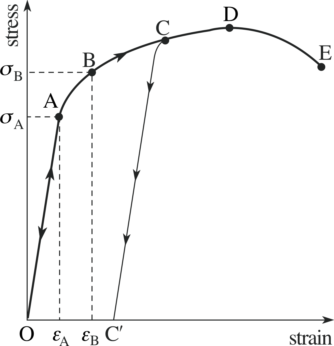
Figure 3 The loading curve of stress against strain for a typical material.
Figure 3 shows the curve representing stress against strain for a typical material. This relationship is known as the loading curve, since it depicts the behaviour of the material under the load of an applied force. (Note that the independent variable is taken to be the strain, although the stress is the physical cause.)
The region from O to A is the region in which the strain is proportional to the stress; this is the range of validity of Hooke’s law. Between A and B the material continues to behave as an elastic material, in that its strain would return to zero if the stress were removed, but stress and strain are no longer related linearly. The elastic region is from O to B, where stress and strain are uniquely related, the behaviour is reproducible and, if the stress is reduced, the material moves back along the curve to its previous state.
Thus, if we apply a stress and measure the strain εA (corresponding to σA), then increasing the stress to σB will produce the larger strain εB. If we then reduce the stress back to σA, we will find that the strain is again εA. The point B, which marks the end of the elastic region, is called the elastic limit or yield point.
Question T4
Consider the loading curve shown in Figure 3. If the measured values associated with point A are εA = 10−3 and σA = 2 ×10⁸ N m−2, what would be Young’s modulus for this material?
Answer T4
SinceσA = YεA, therefore:
$Y = \dfrac{\sigma_{\rm A}}{\varepsilon_{\rm A}} = \rm \dfrac{2\times10^8\,N\,m^{-2}}{10^{-3}} = 2\times10^{11}\,N\,m^{-2}$
If the stress is increased beyond point B, the material enters the plastic region or ductile region. This region is characterized by the material exhibiting plasticity and having large increases in strain resulting from relatively small increases in stress. In the plastic region the material becomes permanently deformed. For instance, if the material reaches the point C and then the stress is reduced the material does not retrace the loading curve but will remain strained, maintaining the value of strain at C′ even in the absence of stress.
If the loading curve is extended beyond point D then the state becomes time–dependent and the strain will continue to increase without further increase in stress. This phenomenon is known as creep. At this stage the strain will continue to increase even if the stress is reduced, as shown by the downward part of the curve beyond D. Finally at point E, the breaking point (or maximum stress), the specimen breaks apart. We will discuss this further in the next subsection.
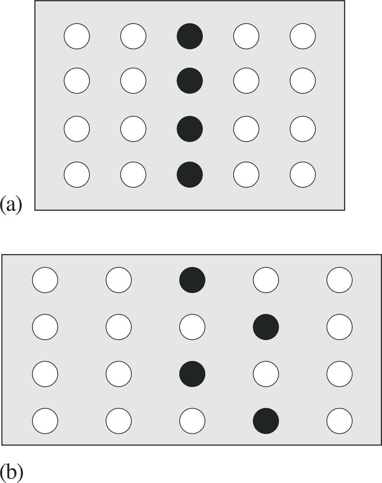
Figure 4 (a) Chains of atoms in a rod before elastic strain, showing a marked plane of atoms. (b) The same rod under a plastic strain. The chains have slipped with respect to each other.
How can we understand the phenomenon of plastic behaviour? We modelled elastic behaviour in terms of rows of atoms connected by springs, with the springs being stretched as the stress is applied to the material. This is clearly a crude picture but it captures the essence of the solid, if we keep in mind that the springs represent more complicated electrostatic forces acting between the atoms.
Figure 4 shows schematically what happens beyond the elastic limit. Figure 4a shows the material without applied stress; one plane of atoms has been identified by filled circles. In Figure 4b the strain has been increased into the region of plasticity and the individual chains of atoms have slipped past each other. Atoms which were formerly neighbours are no longer neighbours. Note that the macroscopic structure of the rod has changed. Now, it is longer (strained); when the stress is relieved the atomic chains do not slip back to their original position. Instead, the atomic springs regain their original lengths but the overall rod length has increased (the deformation is permanent). Note that there is no way of applying a macroscopic force to push the chains back to their original configuration. This is only a simplistic picture of what occurs when a material exhibits plastic behaviour; it certainly leads to no quantitative understanding or predictions, but it gives some insight into how permanent deformation can occur at the microscopic level.
2.3 Brittleness and fracture
A material can be characterized by the nature of its loading curve, which depends critically not only on the chemical composition, but also on the existing microstructure. This is the actual structure of the material at the microscopic level and includes not only the idealized positions of the atoms but also the presence of impurity atoms and defects (missing atoms or holes in the atomic lattice). This microstructure can be drastically altered by treatment of the material such as cold working (repeated controlled stressing of the sample) or annealing (controlled heating and cooling of the sample).
✦ As an example of cold working, take a paper clip and straighten it out; then bend one section back and forth a number of times. What happens?
✧ At first, it can be bent back and forth with little permanent change, although it may feel a bit warmer right at the bending point. If you continue this, eventually (after perhaps 10 or 15 cycles), the section will snap, even though any individual bending motion is well within the original capability of the metal wire.
This application of repeated stress has shifted the breaking point of the material.
Figure 3 The loading curve of stress against strain for a typical material.
Figure 3 shows a general loading curve; however, the relative size of the different regions and the shape of the curve can vary dramatically. In particular, the region from B to E can be very large in some materials (for example in polymers such as rubber) or almost non–existent (for example in glass or concrete). In the latter case, the material is said to be brittle, or to exhibit brittleness, and tends to fracture soon after (or even before) it reaches its elastic limit, rather than deforming. Brittle materials are not necessarily weak materials. Brittleness means that the material fractures before or very soon after exceeding the yield point (in other words, that the range of strains between the yield point and the fracture point is small by comparison to the strain at the yield point); the actual value of stress may be very high at that point. Weak materials break under small stresses but the range of strains constituting the plastic region may still be large, so that it extends well beyond the yield point before reaching the breaking point.
Thus far we have concentrated on tensile stresses, where the forces extend the body. Similar considerations apply to situations where the body is compressed. If the forces applied to a rod are directed inward to compress the rod along its axis, then we have uni–axial compressional stress and uni_axial_compressional_strainstrain.
This is conceptually similar to tensile stress and strain, but the stress and strain have the opposite sign. For both tensile stress and compressional stress it is the Young’s modulus which describes the response of the body.
2.4 Shear modulus and bulk modulus
There is another class of stress on a body, in which non–collinear forces twist the body and change its shape. This is called a shear stress and is illustrated in Figure 5. Here a rectangular section block is subject to two balanced forces of equal magnitude, applied uniformly to two separated surfaces. The forces are applied parallel to the surfaces, rather than perpendicular to the surfaces as in tensile stress, and this twists the block and changes its shape.
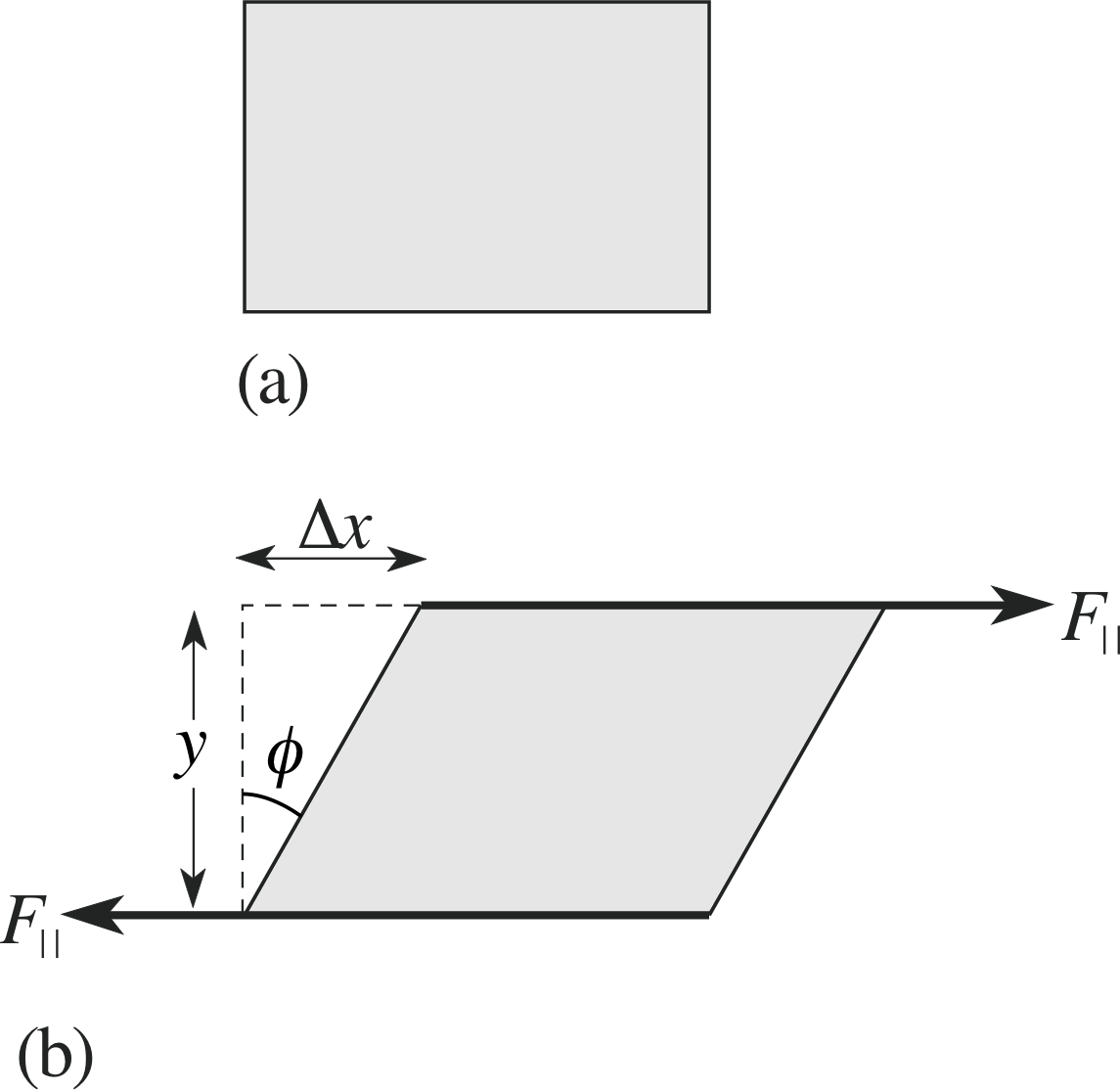
Figure 5 Non–collinear forces applied to a rectangular block (a) lead to shear stresses and a distortion of its shape (b). These shear forces would tend to impart a rotational motion to the block, so that other forces must be applied to prevent the rotation. In this discussion we ignore these other forces.
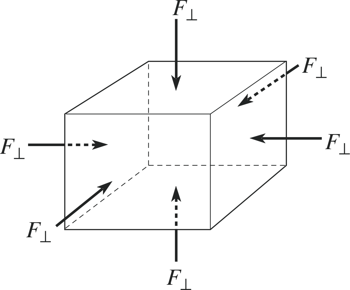
Figure 6 A uniform volume stress (uniform pressure) applied to a body.
Just as for tensile stress, the shear stress is defined as the ratio of the applied force to the area over which it is applied, remembering that in this case the forces are applied parallel to the surfaces, we represent it as F|| and write:
shear stress $\sigma_{\rm S} = \dfrac{\text{magnitude of parallel force}}{\text{area of surface of application}} = \dfrac{F_{||}}{A}$(4)
The shear strain is defined as the ratio of the shear distance between the two surfaces, measured parallel to the applied stress, to the perpendicular distance between the two surfaces. In Figure 5b, these are denoted by ∆x and y, respectively. So, in this case the shear strain is calculated as:
shear strain $\varepsilon_{\rm S} = \dfrac{\text{shear between the two surfaces}}{\text{separation between the two surfaces}} = \dfrac{\Delta x}{y}$(5)
Notice that the shear strain is dimensionless, since it is the ratio of two distances. Also, since these strains are generally very small, we can say that the angle of the shear (denoted by ϕ) is equal to the shear strain, since ∆x /y = tan ϕ ≈ ϕ (measured in radians) for small angles. As with tensile stresses and strains, for small stresses and deformations the shear strain is linearly proportional to the shear stress and we can define a shear modulus G by:
shear modulus $G = \dfrac{\text{shear stress}}{\text{shear strain}} = \dfrac{\sigma_{\rm S}}{\varepsilon_{\rm S}}$(6)
Finally, we will consider a third type of stress, a uniform stress or a volume stress. In this case the force is applied to the body uniformly, perpendicular to every surface, as shown in Figure 6. The magnitude of such a stress is usually called a pressure. The pressure on a body tends to compress it and reduce its volume. Pressure itself is a scalar quantity which cannot be negative, so it is incorrect to speak of the direction of a pressure; however, the forces applied to a body due to pressure on the body do have a direction – and this is into the body. The pressure is numerically equal to the perpendicular force per unit area of the surface of the body.
volume stress (pressure) $\dfrac{\text{magnitude of perpendicular force}}{\text{area of surface of application}} = P$(7)
The resulting strain is normally a volume strain, and is calculated as:
volume strain $\varepsilon_{\rm vol} = \dfrac{\text{change in volume}}{\text{total volume}} = \dfrac{\Delta V}{V}$(8)
The volume always decreases with increase of pressure and so ∆V is negative, as is the volume strain. The elastic modulus corresponding to volume stress and strain is called the bulk modulus K, which is defined as:
bulk modulus $K = \dfrac{\sigma_{\rm vol}}{\varepsilon_{\rm vol}} = - \dfrac{\text{pressure change}}{\text{ fractional volume change}} = -V\dfrac{\Delta P}{\Delta V}$(9)
Notice that, by convention, we use ∆P for the stress, since it is normally taken that the reference state is atmospheric pressure (rather than zero pressure) and we require the minus sign since pressure is positive.
| Material | Y / 1010 N m−2 | G / 1010 N m−2 | K / 1010 N m−2 |
|---|---|---|---|
| aluminium | 7.0 | 2.5 | 7.5 |
| copper | 11.0 | 4.4 | 13.5 |
| steel | 20.0 | 7.5 | 17.0 |
| nylon | 0.36 | 0.12 | 0.59 |
These different elastic moduli represent the response of a material to different forms of external stress, but all are ultimately based on the same interatomic forces, and so one would expect their values to be linked.
Table 2 shows typical values of the elastic moduli for some common materials.
Question T5
A shear stress of 1.0 × 10⁵ Pa is applied to samples of each of the materials in Table 2. Which will exhibit the largest shear strain and what will be its value?
Answer T5
Since σS = GεS and $\varepsilon_{\rm S} = \dfrac{\sigma_{\rm S}}{G}$, the smallest value of the shear modulus will produce the largest shear strain.
This will be for nylon, with G = 0.12 × 10¹⁰ N m−2.
Therefore:
$\varepsilon_{\rm S} =\rm \dfrac{1.0\times10^5\,Pa}{0.12\times10^{10}\,Pa} = 8.3\times10^{-5}$
3 Fluidity
Fluids are distinguished from solids in that they have no fixed shape, but (under the influence of gravity) adopt the shape of any container; in other words, they flow. Both gases and liquids are fluids, but gases tend to expand to fill the available volume, while liquids tend to have a fixed volume.
This can be understood in terms of the much stronger intermolecular forces between molecules in a liquid than those in a gas. In solids these forces are even stronger and so a solid also tends to maintain its shape. Here we will be concerned mainly with the properties of liquids. In the terms we have introduced so far in our discussion of solids, we can characterize fluids by saying that they cannot sustain tensile, uni–axial compressive or shear stresses in equilibrium. Let us look at this claim a little closer.
First, if we apply a tensile stress to a given quantity of liquid, i.e. try to pull it apart from two sides, the liquid will simply come apart on us. The attractive forces between the molecules are generally not sufficiently strong to hold the liquid together under tension (although see Subsection 4.4 for further discussion of this).
Secondly, if we could somehow have a column of liquid free of a container (say in the absence of gravity) and we tried to apply uni–axial compression forces to the two ends, then the liquid would simply squirt out sideways. Another way of making this point is to say that one cannot grab a piece of liquid.
Finally, while solids under a shear stress will distort slightly, then maintain the new shape (with the external shear forces balanced by internal elastic stresses), fluids will continue to distort under a shear, maintaining a constant rate of displacement. The consequence of this is that, in equilibrium, only a uniform stress can be present in a liquid.
As mentioned earlier, this uniform stress is commonly known as pressure. In this section, we will consider only the equilibrium properties of liquids; also we will consider only the simplest example of liquids, those which are said to be incompressible. This implies that when a pressure is applied to such a liquid, the volume change can be taken to be zero. This condition is certainly not true for a gas but it is a very good approximation for most liquids, when subject to usual pressures. It is only approximately true since its strict truth would imply an infinite value for the bulk modulus.
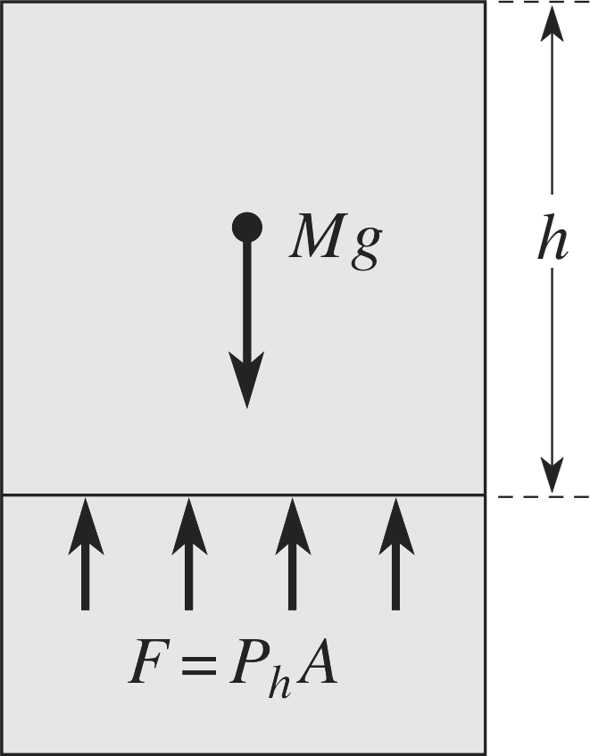
Figure 7 At any particular level in a liquid, the hydrostatic pressure must balance the weight of liquid above that level, in order for equilibrium to exist.
3.1 Hydrostatic pressure
As discussed above, the only stress that can be present in a fluid in equilibrium is the uniform stress called pressure. We can consider two sources of pressure in a liquid. The first is due to the force of gravity on a column of liquid, which in the absence of a balancing force would cause the liquid to fall. In fact, the weight of the liquid above a given height produces the hydrostatic pressure Ph of the liquid at that height, as indicated in Figure 7. This means that we can write the hydrostatic pressure as a function of the height of the column of fluid above it. If we take a column of liquid of mass density ρ and cross–sectional area A then the equilibrium at depth h gives Mg = Ahρg = Ph A with the
hydrostatic pressure Ph = ρgh(10)
We see that in any connected volume of fluid the pressure must be the same at the same height, or else the fluid would not be in equilibrium. We also see that in the absence of gravity, this internal hydrostatic pressure vanishes.
Question T6
In the Pacific Ocean, the Marianas trench reaches a depth of 11 033 m (the deepest part of any ocean).
What is the hydrostatic pressure at the bottom of this trench?
(Take the density of sea water to be constant at 1027 kg m−3).
Compare this to ordinary atmospheric pressure, which is 1.01 × 10⁵ Pa.
Answer T6
We use:
Ph = ρgh = 1027 kg m−3 × 9.81 m s−2 × 11 033 m = 1.11 × 10⁸ Pa
This is 1.11 × 10⁸ Pa/(1.01 × 105 Pa) = 1.10 × 10³ atmospheres
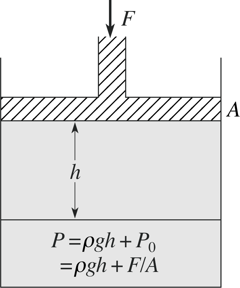
Figure 8 An external force applied to a fluid produces an additional pressure.
3.2 Pascal’s principle
In addition to the hydrostatic pressure, there is also the pressure resulting from external stresses, which might be applied by some sort of piston, for example, as shown in Figure 8. How does this external stress affect the pressure within the fluid?
The answer is given by Pascal’s principle: i
Any external pressure is transmitted uniformly to every element of the fluid, and hence to the walls of the container.
This implies that at every point in a fluid (at the same height), the pressure will be identical.
Question T7
In the apparatus shown in Figure 8, a force of magnitude 100 N is applied to a piston of area 10.0 cm2. If the liquid is mercury, with a density of 1.355 × 10⁴ kg m−3, what will be the total pressure 15.0 cm below the piston?
(Ignore atmospheric pressure.)
Answer T7
The total pressure will be given by
P = Ph + Pext = ρgh + F/A
soP = (1.355 × 10⁴ kg m−3 × 9.81 m s−2 × 0.150 m) + [100 N/(10−3 m2)]
P = (1.99 × 10⁴ Pa) + (1.00 × 10⁵ Pa) = 1.20 × 10⁵ Pa
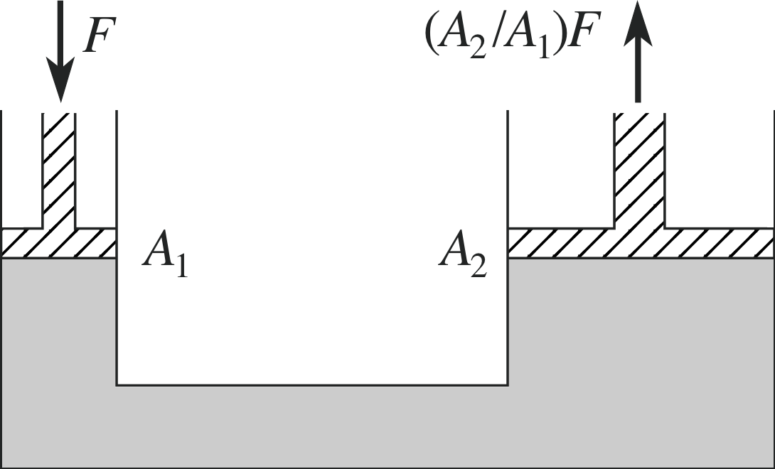
Figure 9 A force applied to the small piston on the left leads to a much larger force produced on the large piston on the right.
This principle also allows us to use fluids to amplify an applied force, as is illustrated in Figure 9. Here a force of magnitude F is applied to the small piston of cross–sectional area A on the left–hand side of the apparatus. This produces a pressure on the fluid equal to F/A, which by Pascal’s principle must be the same as that at the equivalent height on the right–hand side.
This pressure then results in a force on the right–hand piston whose magnitude is equal to P × A2 = F × (A2/A1), so that the magnitude of the applied force has been amplified by the ratio of the cross–sectional areas. This technique is used, for example, in the hydraulic braking system of a car; a small force at the brake pedal is transmitted through the brake fluid to appear as a large force applied through the brake pads at the wheels.
3.3 Archimedes’ principle and buoyancy
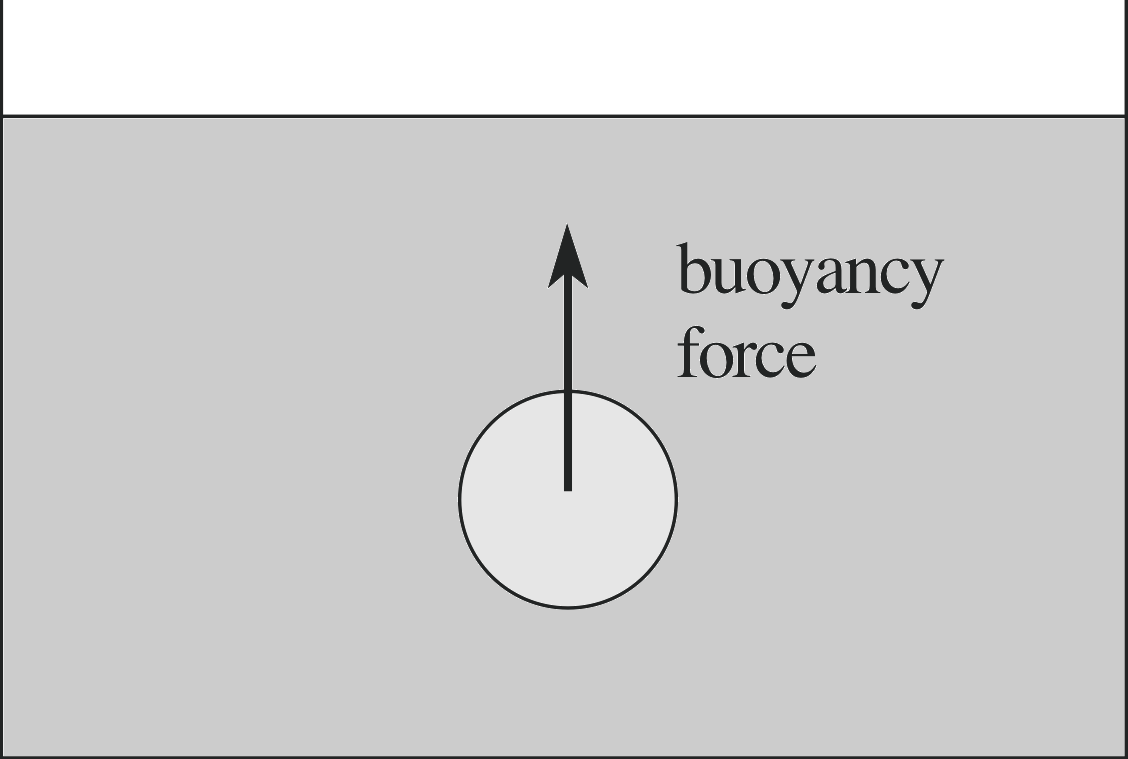
Figure 10 A body immersed in fluid experiences a force due to the surrounding fluid that is equal to the weight of the displaced fluid.
When an object is immersed in a fluid, it must displace a volume of fluid equal to the volume of the object immersed. We start by considering a body completely immersed, as shown in Figure 10.
If we assume that the state of the remaining fluid is unchanged by the replacement of fluid by the solid body then the force exerted by the remaining fluid on the solid body must be the same as the force which this fluid had previously exerted on the displaced fluid. We know that this force was a net upward force equal to the weight of the displaced fluid, since this fluid was previously in equilibrium. It is apparent then that a body within a fluid must experience a net upward force which is exactly equal in magnitude to the weight of the fluid which the body has displaced.
This is known as Archimedes’ principle, which we can state as follows: An object immersed in a fluid will experience a net force due to the fluid which acts upward, with a magnitude equal to the weight of the fluid displaced by the object.
The process by which a fluid tends to support an immersed object is called buoyancy and the upward force on the object due to the fluid is called the buoyancy force (sometimes also called the upthrust). The resultant force on the immersed object will be the difference between the downwards force due to gravity (its weight) and the upward buoyancy force from the fluid that surrounds it. If the weight exceeds the maximum buoyancy force, produced when the object is fully immersed, then the object will weigh less than in air, but will still sink in the fluid.
If the weight can be balanced by the buoyancy force, with the object partially immersed, then the object will float in equilibrium with this fraction of the body immersed. In this second case, if the object is then fully immersed in the fluid by the application of some other external force, it will rise up through the fluid if this force is removed. A sinking object behaves as if its weight were less than in a vacuum, a floating object behaves as if it were weightless, and a released rising object behaves as if it had a negative weight! i Notice that, like the weight itself, the buoyancy force requires the presence of gravity.
✦ Suppose we have a small experimental system such as in Figure 10, with an object which just floats in a certain liquid. We now transport this system to Mars, where the surface gravity is 0.38 that on Earth. Assuming that nothing other than the force of gravity changes, what would happen to the object?
✧ There would be no change. The force of gravity and the buoyancy force would both change by the same ratio, so the object would still just float.
Question T8
An astronaut in a stable Earth orbit takes a glass of water and pushes down a cork to the bottom of the glass with her finger. What happens to the cork when she removes her finger, assuming that the water stays in the glass?
Answer T8
Assuming the water stays in the glass, the cork would remain fully submerged. In the stable orbit weightless conditions prevail.
4 Surface effects and interfaces
So far our discussions have concentrated on solids and fluids as if they were uniform materials, with no boundaries. In fact this is a highly idealized model. Real materials have boundaries and there are important processes which come into play at these boundaries and particularly at the boundaries or interfaces between two different materials. You will already be aware of several of these processes. For example, the friction between two contacting sliding surfaces is one such case and air resistance is another. We begin with a discussion of friction.
4.1 Friction and its atomic basis
Friction is a familiar force from elementary mechanics and real life. Our ability to move around depends on the existence of friction, but it is a rather unusual force. It is generally classified into two types, static friction and sliding friction, with the distinction being based upon whether or not the two surfaces experiencing the frictional force are sliding across each other. An example of static friction might be of a car parked on a hill, whilst sliding friction comes into play when the car skids. You might be surprised to hear that it is static friction which allows the car to negotiate a bend safely, without skidding, since the rolling of the tyres along the road (without sliding) is governed by static friction.
At the macroscopic level, the behaviour of the friction force between two unlubricated solid dry surfaces can be described fairly simply by the following empirical laws, discovered independently by Leonardo da Vinci (1452–1519) and Guillaume Amontons (1663–1705).
- 1
-
The friction force is proportional to the reaction (normal) force pressing the surfaces together.
- 2
-
The friction force is independent of the macroscopic area of contact for a given reaction force.
- 3
-
If two surfaces are caused to slip, the friction force is independent of the relative speed between the two surfaces, once relative motion has occurred, but less than that just before the relative motion occurs.
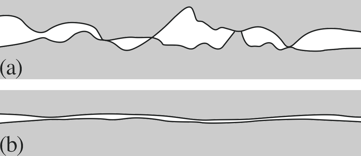
Figure 11 Two interfaces exhibiting contact friction: (a) a typical surface which is rough on the microscopic scale, and (b) a surface which is smooth, even at the microscopic level.
These empirical laws describe the basic observations, but there are many exceptions and the real situation is much more complex.
The first of these laws seems reasonable and accords with experience – it is much harder to push a loaded car than an empty car.
You probably find the second law to be rather unexpected. The explanation for it is that the friction force is determined by the microscopic, not the macroscopic, contact area. At a microscopic level, all surfaces show marked irregularities. When two surfaces are in ‘contact’ they meet only at the peaks of these irregularities (Figure 11a) and the real contact area is very much less than the apparent macroscopic contact area. As we spread the weight there are more, but less deformed, contact regions and the microscopic contact area is left more or less unchanged.
As the weight (or any other normal force pushing the two surfaces together) increases, the amount of microscopic contact will increase due to local strains on the projections on the surfaces, which accounts for the usual dependence on the normal reaction force.
On a microscopic level the friction force arises from the interaction between the layers of atoms in close contact. One simple model for this process of contact friction postulates that the force can be expressed in the form
f = σmaxAreal(11)
where σmax is the maximum shear strength of the weakest material forming the contact, and Areal is the real microscopic area of contact. The largest component of the friction force is due to the adhesion of these microscopic contact areas. A striking example of the increase of friction by increasing the microscopic contact area occurs where two surfaces are specially polished so that they are almost flat on a microscopic scale (Figure 11b). The friction between the surfaces is greatly increased by the polishing, which may surprise you, as polishing usually reduces the friction – but not if the surfaces become flat on a microscopic scale. You may have seen this increased friction with two sheets of glass in contact. In the limit, where the two surfaces are made sufficiently flat, they may even bond together on contact; the adhesion forces between the surfaces are then so strong that any attempt to move one object with respect to the other amounts to shearing a single solid object. i
Other mechanisms are believed to play a smaller part in the case of contact friction. When two surfaces slide across each other, the rough spots (asperities) tend to collide, causing local deformations. Some of these deformations will be elastic and others may lead to permanent deformations (gouges) in the microscopic surface and to the dissipation of energy into heat. The larger the normal force pushing the two surfaces together, the more significant are these deformations and the more energy will be dissipated in the motion.
The third law is also in accord with experience. It takes a certain minimum applied force to start a body sliding over a horizontal surface, but once sliding starts, a smaller applied force is enough to keep the body moving at constant velocity – any driver who has braked on ice or taken a bend too quickly, knows this very well! If we apply a horizontal force to a stationary body lying on a horizontal surface, but the body does not move, then the friction force on the body must have the same magnitude as the applied force. As this force is increased, the opposing friction increases to match it exactly until a critical value is reached. When the applied force is increased still further the body starts to slide and the magnitude of the friction force falls rapidly to a lower value and then remains reasonably constant. Experiments show that the third law breaks down for very high speeds, when the frictional force reduces slightly.
The first law suggests that the friction between two surfaces can be characterized by defining a coefficient of friction, as the ratio of the magnitudes of the maximum frictional force and the reaction force. The third law implies that these maximum forces are different for static and sliding friction and so we need to define a coefficient of static friction μstatic and a coefficient of sliding friction μslide.
The first law of friction, telling us that the magnitude of the friction force is proportional to the magnitude of the reaction force R, allows us to define these two coefficients of friction:
μstatic is defined by: (fstatic)max = μstatic R(12) i
μslide is defined by: (fslide)max = μslide R(13)
Since both these coefficients relate the magnitudes of two forces, they are dimensionless quantities. Since it takes a larger force to start a body moving than to keep it moving it is clear that, in general, μstatic > μslide. For example, with rubber on tarmac μstatic ≈ 1 while μslide ≈ 0.7.
It should be remembered that the above description is an oversimplification. The real area of contact may be increased if one of the materials is readily deformable, such as is generally true for polymeric materials like rubber. For example, tyres are designed to provide a large amount of real contact area with the road. According to the above simple description of friction, the road–holding and braking ability would be the same for a standard car tyre as for one the size of a bicycle tyre – but that clearly is not true.
Question T9
Suppose a block of aluminium sits on a level steel surface. The block has a contact surface of area of 4.0 cm2, a mass of 20 g, and the ordinary coefficient of static friction between the aluminium and steel is 0.61. If the maximum shear strength is 2.0 × 10⁷ Pa, what is the actual microscopic area of contact between the two surfaces in the adhesion model? What fraction of the apparent contact area is this?
Answer T9
Equation 11,
f = σmaxAreal(11)
givesf = σmaxAreal
Equating this to f = μstaticR we have:
$A_{\rm real} = \dfrac{\mu_{\rm static}R}{\sigma_{\rm max}} = \rm \dfrac{0.61\times0.02\,kg\times9.8\,m\,s^{-2}}{2.0\times10^7\,Pa}$
soAreal = 0.12 N/(2.0 × 107 N m−2) = 6.0 × 10⁻⁹ m2
This is a fraction of the apparent contact area, given by
6.0 × 10⁻⁹ m2/(4.0 × 10−4 m2) = 1.5 × 10⁻⁵
i.e. fifteen millionths.
4.2 Viscosity and its atomic basis
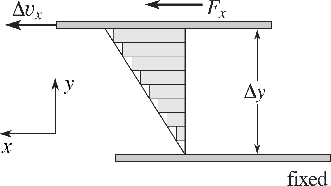
Figure 12 A fluid is contained relative motion. The rectangles indicate the velocity profile of the fluid with respect to the bottom plate.
Viscosity is a property of a fluid which is used to characterize its resistance to flow under applied forces. If we consider the difference between water and treacle, and note that treacle is more viscous, then the concept is quite familiar. Viscosity can be thought of as internal friction in a fluid, which acts both between a fluid and a bounding solid surface and between internal elements of the fluid itself. In order to define viscosity more precisely, we need to examine a fluid under shear stress.
We’ve remarked already that a fluid cannot sustain a shear stress in between two parallel plates in uniform equilibrium, so we see that we are going to be considering non–equilibrium situations. However, to keep life simple, we will consider only steady-state conditions, in which the fluid moves or flows at a steady rate but the overall state of the system does not change with time. The system is said to be in dynamic equilibrium.
Figure 12 shows a standard geometry for analysing viscosity. We consider fluid contained between two parallel plates in relative motion, separated by a distance ∆y. We take the bottom plate to be at rest, with the top plate moving uniformly at a velocity ∆υx with respect to it. For moderate relative velocities, the flow of the liquid between the two plates will be smooth, with a uniform change in velocity (relative to the bottom plate) from zero up to ∆υx. This velocity profile is displayed in the figure. Notice that the fluid in contact with each solid surface has the characteristic velocity of that surface.
The motion of the top plate will require a constant force to overcome the effects of viscosity (or friction), which would otherwise slow down and prevent the relative motion. To maintain the motion we will require a force Fx applied to the plate. If the fluid flow is not too high the flow will be smooth, rather than turbulent, and we then find that the force increases linearly with the velocity gradient in the fluid and with the area of the plate. We can then characterize the viscosity of the fluid by defining a coefficient of viscosity η (often simply called the viscosity) by the expression: i
viscous force $F_x = \eta A\dfrac{\Delta\upsilon_x}{\Delta y}$(14)
This can also be expressed in terms of a viscous shear stress as:
viscous shear stress $\sigma_x = \eta\dfrac{\Delta\upsilon_x}{\Delta y}$(15)
✦ What must be the units of the coefficient of viscosity as a combination of fundamental SI units, i.e. in terms of kg, m and s?
✧ In order for this equation to be dimensionally consistent, the coefficient of viscosity must have SI units of kg m−1 s−1. This is equivalent to N m−2 s, or Pa s.
In addition to the SI units of ‘pascal seconds’, viscosity is often expressed in units of poise, defined as 1 poise = 10−1 Pa s.i
| Liquid | η/10−3 Pa s |
|---|---|
| glycerine | 830 |
| mercury | 1.58 |
| olive oil | 84 |
| water | 1.01 |
Everyday fluids cover a wide range of viscosities (consider the difference between water and treacle again), typically between 10−5 Pa s (for gases) and 1 Pa s (glycerine, for example). On the other hand, flowing lava can have a viscosity of 104 Pa s, and the viscosity of glass at room temperature can be of the order of 1018 Pa s (yes, glass can flow, though you have to wait a very long time to detect the flow under its own weight!). Table 3 gives values of the viscosity for some common liquids.
This linear relationship between the force and the velocity gradient is only an approximation for some fluids under some circumstances. Fluids for which this relationship holds are known as Newtonian fluids, since Newton first presented this description of such flows. This relationship will break down outside certain limits, in this case if the velocity gradient becomes too high or the flow becomes turbulent. In addition, complex fluids that are suspensions or dispersions of particles in liquids are frequently non–Newtonian (interesting examples are blood and paint).
Figure 12 A fluid is contained between two parallel plates in uniform relative motion. The rectangles indicate the velocity profile of the fluid with respect to the bottom plate.
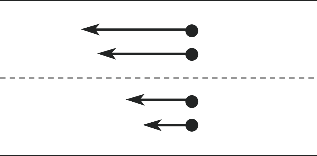
Figure 13 Imaginary surface (dashed line) in a fluid under shear. Fluid molecules above the surface have a larger transverse velocity than those below the surface.
At the microscopic level there are two mechanisms responsible for viscosity in fluids. The first of these tends to dominate in gases, while the second is more important in liquids.
To appreciate the first mechanism, look again at Figure 12. Consider an imaginary surface in the fluid, parallel to the boundary plates as indicated in Figure 13. The fluid elements above this surface have a higher x–component of velocity than fluid elements below the surface. However, this refers to the bulk motion of the fluid. In reality, both in gases and liquids, the atoms or molecules are in a state of constant random motion at the microscopic level. Any bulk flow motion is superimposed on this random motion. Therefore, across any such imaginary surface in the fluid, there will be molecules moving up or down and on average they will have the bulk velocity of the fluid layer from which they came.
Molecules moving upward through the surface will carry with them an average x–component of momentum which is less than that of the molecules within the layer they are joining. Collisions with the molecules in this layer will, on average, increase their x–component of momentum but, by the principle of conservation of momentum, will reduce the average x–component of momentum of the other atoms in this layer. This implies that the upper layer will have its average x–momentum reduced by the ingress of the molecules from below. A similar argument, applied to molecules moving down through the surface, will lead to a net increase in the x–component of momentum of the layers below. This process of momentum transport between the layers thus acts to decrease the relative motion between the layers, in other words, to produce a drag force. This transfer of momentum between layers is the main cause of viscosity in gases.
This same mechanism also operates in liquids but the transport of momentum between layers is less significant here. Molecules do not move so easily between layers because of the shorter average distance between collisions (or the shorter mean free path) in a liquid. The more important consideration in liquids arises directly from the larger attractive forces between the molecules. These forces are strong but they have a very short range, extending over only one or two molecular diameters, so the molecules are aware only of their nearest neighbours. From Figure 13 we can see that attractive forces between the molecules in adjacent layers will act on average to slow the molecules in the layer above the surface and speed up those below the surface. It is these attractive forces, operating across shearing layers, which are the primary cause of viscosity in liquids.
4.3 Stokes’ law, terminal speed and air resistance
The resistance that a solid body feels when it moves through a fluid medium (such as a car moving through the air) is a very complicated phenomenon, depending on the shape of the body, the nature of the fluid medium, and the relative speed of the body through the medium. For small relative velocities, it is found that a good approximation to the drag force on a sphere is given by Stokes’ law:
Stokes’ law Fx = −6πaηυx(16) i
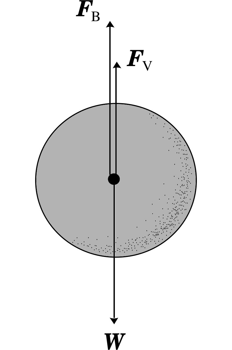
Figure 14 A sphere falling through a viscous fluid experiences three forces: the force of gravity (W), the buoyancy force (FB) and the drag force (Fv). The two upward acting forces have been displaced for clarity.
Here η is the viscosity of the fluid, a is the radius of the sphere, and υx is the relative velocity of the sphere through the fluid. The negative sign signifies that the force opposes the motion. Since this resistive force is proportional to the relative velocity of the body, if a body falls under its own weight through a fluid, this velocity will only increase until the force of gravity is balanced by the drag force due to Stokes’ law. At this point, the velocity will stay constant for the remainder of the fall. The velocity at which this occurs is known as the terminal velocity.
Consider the falling sphere shown in Figure 14. The forces acting on it are the force of gravity W, the buoyancy force FB due to the displaced fluid, and the viscous drag force Fv. If we assume that the sphere has reached its terminal velocity, υt, then the acceleration will be zero, which means that the net force on it must be zero. We take ρsphere to be the density and V the volume of the sphere, with ρfluid as the fluid density. Then:
W + FB + Fv = 0 where 0 is the zero vector
In terms of the magnitudes of these forces:
W − FB − Fv = 0
or ρsphereVg − ρfluidVg − 6πaηυt = 0
and the terminal velocity is:
$\upsilon_{\rm t} = \dfrac{\left(\rho_{\rm sphere} - \rho_{\rm fluid}\right)Vg}{6\pi a\eta}$(17)
Air resistance is a familiar example of the effects of viscosity in a gas. It is known to any cyclist or motorist and is of more than passing interest to parachutists. It is of such technological importance in today’s world that it has been studied in great detail. Experimentally it is found to vary with the profile presented to the air flow and with the size and relative speed of the moving object.
For spheres of radius a moving at speed υ through still air it is found that the frictional force obeys Stokes’ law at low speeds, being proportional to aυ when aυ < 10−4 m2 s−1 (streamlined flow of the air). At higher speeds the force is proportional to a2υ2 (turbulent flow of the air). At very high speeds (aυ > 1 m2 s−1) the dependence is even more complicated. Most everyday objects, even though not spherical, display the υ2 dependence, and this is one reason for the pronounced increase in car fuel consumption at high speeds.
Question T10
Verify that the expression on the right–hand side of Equation 17 has the dimensions of velocity.
Answer T10
Density has dimensions M L−3; volume has L3, g has L T−2, radius has L and viscosity has M L−1 T−1.
Therefore the right–hand side of
$\upsilon_{\rm t} = \dfrac{\left(\rho_{\rm sphere} - \rho_{\rm fluid}\right)Vg}{6\pi a\eta}$(Eqn 17)
has dimensions
$\rm \dfrac{M\,L^{-3}\,L^3\,L\,T^{-2}}{L\,M\,L^{-1}\,T^{-1}} = \dfrac{M\,L\,T^{-2}}{M\,T^{-1}} = L\,T^{-1}$
which are the correct dimensions for velocity.
Question T11
Using the fact that the volume of a sphere of radius a is (4/3)πa3, obtain a simplified expression for its terminal velocity.
Answer T11
Substituting for V gives us
$\upsilon_{\rm t} = \dfrac{\left(\rho_{\rm sphere} - \rho_{\rm fluid}\right)Vg}{6\pi a\eta} = \dfrac{\left(\rho_{\rm sphere} - \rho_{\rm fluid}\right)\dfrac{4\pi a^3}{3}g}{6\pi a\eta} = \dfrac{2a^2g}{9\eta}\left(\rho_{\rm sphere} - \rho_{\rm fluid}\right)$
4.4 Surface tension and capillarity
We now turn once more to the short–range attractive intermolecular forces that act in liquids. These are labelled as forces of cohesion if they act between different elements of the liquid itself, and forces of adhesion if they act between elements of the fluid and another material, such as the wall of a container. As discussed earlier, the forces of cohesion acting within the volume of a liquid are primarily responsible for its viscosity. Liquids tend to adopt the shape of their container, but the cohesive forces cause exceptions to this tendency. Small drops of liquid will tend to adopt a spherical shape.
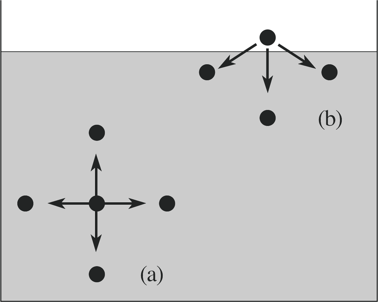
Figure 15 Intermolecular forces in a liquid: (a) a molecule in the interior of the liquid experiences (on average) an equal force of attraction from all sides; (b) a molecule just above the surface has few neighbours on one side, and so feels a net force of attraction towards the surface.
Liquids are also generally unstable under a non–uniform stress, so that if you push on a liquid in just one place (as opposed to a uniform pressure over the entire surface), it will tend to squirt aside. Again, the cohesive forces cause exceptions to this tendency, for very small forces. For example, a surface of a liquid can sustain the weight of small objects like a thin string or an insect. For both these classes of exceptions, the surface acts as a very thin, weak elastic membrane enclosing the liquid. This is the phenomenon of surface tension, which arises from the cohesive forces, and can be understood in terms of an imbalance in these forces on molecules that are attempting to leave the surface of the liquid.
Figure 15 shows that molecules within the liquid (a) experience a balance of forces due to the near neighbour molecules on all sides, but just above the surface of the liquid (b) there is a net attractive force pulling the molecule back into the liquid, since relatively few molecules exist in the vapour phase above the surface.
This net force means that work must be done to expand the surface of a liquid, since that requires pulling more molecules away from near neighbours. In terms of energy, an energy input is required to increase the surface area of the liquid by moving more molecules into the surface. Without this input the liquid will tend to minimize its surface area. For a drop of a given volume the minimum surface area occurs when the drop is spherical. For small drops this is the dominant effect and accounts for the spherical shape of these drops. With larger drops the effects of gravity tend to distort the drops from a spherical shape.
The surface tension γ characterizes the difficulty in increasing the area of a surface. i It is defined as the work done ∆W or the increased surface energy ∆EA when the area is increased by ∆A:
surface tension $\gamma = \dfrac{\Delta W}{\Delta A}=\dfrac{\Delta E_A}{dA}$(18a)
or, using calculus notation: $\gamma = \dfrac{dW}{dA} = \dfrac{dE_A}{dA}$(18b)
This identifies the SI unit of surface tension as J m−2. Since we can also write this unit as N m−1 it is clear that surface tension can also be written as a force per unit length.
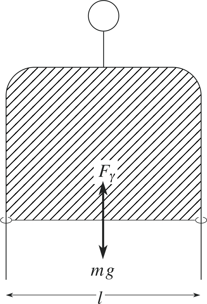
Figure 16 A U–shaped frame with a very light slider holds a thin film.
We can see this with the help of Figure 16, which shows a very convenient method of measuring the surface tension of a film. A thin film is produced within the area bounded by a U–shaped frame and a very light slider (length l), by dipping the assembly into a liquid such as soap solution. If the frame is held vertically, the slider will move up or down until its weight is balanced by the upward force on the slider due to surface tension. If we now displace the slider downwards very slightly through a distance ∆x by applying an external downwards force Fx = − Fγ the film area (two surfaces) increases by ∆A = 2l∆x and the work done is ∆W = Fx ∆x. Equation 18 then gives:
surface tension $\gamma = \dfrac{F_x}{2l}\dfrac{\Delta x}{\Delta x} = \dfrac{F_x}{2l}$(19)
Equation 19 shows that the surface tension is also equal to the magnitude of the force per unit length of the film (two surfaces) in contact with the rider.
Although the SI units for surface tension are N m−1, the typical magnitudes involved mean that values are frequently quoted in mN m−1. In using this definition, it is important to remember that all surfaces must be taken into account. In the system shown in Figure 16, there are two surfaces for the film on the frame, so that if the length of the slider is l the film length is 2l.
Question T12
In an experiment using a liquid and the U-frame, as shown in Figure 16, the mass of the slider is 5.0 mg and its length is 2.0 cm. What is the surface tension of the liquid?
Answer T12
Fγ = 5.0 × 10−6 kg × 9.81 m s−2 = 4.9 × 10⁻⁵ N
2l = 2 × 2.0 × 10−2 m = 4.0 × 10⁻² m
γ = Fγ /(2l) = 4.9 × 10⁻⁵ N/(4.0 × 10−2 m) = 1.2 × 10⁻³ N m−1 = 1.2 mN m−1
| Liquid | γ/10−3 N m−1 |
|---|---|
| glycerine | 63.1 |
| mercury | 475 |
| olive oil | 32.0 |
| water | 72.8 |
Table 4 shows values of the surface tension for some common liquids, although it should be remembered that the actual value depends not only on the liquid, but also on the other material which forms the interface, whether it be a solid or a different fluid. This is because it is the net difference in force between the interior and the exterior of the body of the fluid that produces the surface tension.
The existence of surface tension means that a pressure difference can exist between the two sides of a liquid surface. This is easy to visualize if you imagine the surface tension as producing an effect like a weak elastic membrane, such as with a balloon. A bubble is rather like a balloon except that in a balloon there are elastic stresses within the material of the balloon, while for a bubble the effective stresses all act at surfaces or along edges. Now we will calculate the pressure difference between the inside and outside of such a bubble in air.
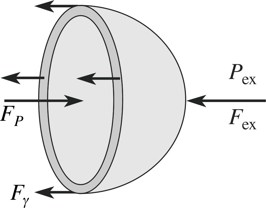
Figure 17 A bubble of liquid in air will have a higher pressure P inside than outside Pex, due to surface tension forces. The force due to the excess pressure on half the bubble is balanced in equilibrium by the surface tension acting along the edge of the hemisphere as shown.
Consider the bubble in air, shown in cross section in Figure 17. We assume that the bubble is in mechanical equilibrium. The pressure P within the bubble must slightly exceed the pressure outside the bubble Pex, otherwise the surface tension forces would cause the bubble to collapse. Suppose the bubble is made to expand its radius from R to R + ∆R by some means (such as by increasing its internal pressure by an infinitesimally small amount). The total surface area of the film (two surfaces) is A = 8πR2 and this will increase by
∆A = 8π (R + ∆R)2 − 8πR2 = 8π (2R∆R) = 16πR∆R
neglecting the term in (∆R)2 which is very small. Equation 18a
surface tension $\gamma = \dfrac{\Delta W}{\Delta A}=\dfrac{\Delta E_A}{dA}$(Eqn 18a)
then gives the required work done to be ∆W = γ ∆A.
This work done can also be calculated from the product of the net force acting radially outwards across the film, FR = (P − Pex) A′ where A′ is the area of the inner surface across which the pressure difference acts.
Since A′ ≈ A = 4πR2 we have FR ≈ (P − Pex) 4πR2, and the distance over which this force acts is ∆R.
So, we have:
∆W = γ ∆A = 16πγR∆R = FR ∆R = 4π (P − Pex) R2∆R
Thus
excess pressure $P - P_{\rm ex} = \dfrac{16\pi\gamma R\Delta R}{4\pi R^2\Delta R} = \dfrac{4\gamma}{R}$(20)
Study comment Although we originally assumed an expansion of the bubble by ∆R in the above argument, the final expression for the pressure difference does not involve this quantity and so is valid without any real expansion of the bubble or any real work done. This type of argument is an example of the principle of virtual work.
Precisely the same reasoning will apply for the situation of a drop of liquid in air or a bubble of vapour within a liquid, with one crucial difference.
✦ In the above discussion, where would the analysis for a liquid drop differ from that for the bubble?
✧ The only difference is that the drop has only one surface, instead of the two that contribute for the bubble in air.
Thus$(P - P_{\rm ex}) = \dfrac{2\gamma}{R}$ for a liquid drop.
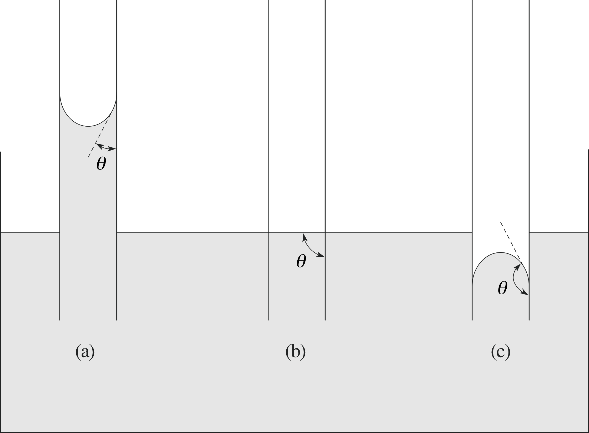
Figure 18 A tube with a small diameter is pushed into a surface of a liquid. (In the figure, the diameter of the tube has been greatly exaggerated for the sake of clarity.) Three outcomes are possible: (a) the liquid rises in the tube; (b) the liquid remains at the original surface level in the tube; (c) the liquid is depressed in the tube.
Finally, we come to another important aspect of the forces that act at interfaces with liquids, that of the capillary effect or capillarity. This is illustrated in Figure 18.
As seen in the figure, three situations can result from a small–diameter tube being pushed into a surface of a liquid: the liquid may rise in the tube, or stay at the original level, or be depressed to a lower level in the tube. The actual result depends on the balance between the forces of surface tension at the liquid–wall, liquid–vapour and vapour–wall interfaces, and the additional force of adhesion between the liquid molecules and the wall molecules.
This means that the actual capillary effect depends crucially on the precise materials of the wall and liquid, so that both must be specified when discussing the effect. The actual physics is quite complicated, but from a descriptive point of view, we can classify the capillary effect in terms of the angle of contact that the surface of the liquid, or meniscus, makes with the solid wall. This angle θ is measured from straight down along the wall, and has a value between 0 and 180°. If θ < 90°, the liquid will rise in the tube, and it is said that the liquid wets the surface of the tube. On the other hand, if θ > 90°, the liquid will be depressed in the tube, and it is said that the liquid is non-wetting with the surface of the tube. Finally, if θ = 90°, the level of the liquid doesn’t change, and it stays at the original position as the tube slides into the liquid.
The force equilibrium sets the surface tension force, acting around the inner circumference of the tube at an angle θ, as being responsible either for supporting the weight of the risen column of fluid or for depressing the fallen column of fluid. If h is the distance the liquid surface rises (or falls) in the tube with respect to the original surface level, γ is the surface tension, θ is the angle of contact, ρ is the density of the liquid, g is the acceleration due to gravity, and r is the radius of the tube we have force equilibrium if:
2πrγ cos θ = πr2hρg
or$h = \dfrac{2\pi r\gamma\cos\theta}{\pi r^2\rho g} = \dfrac{2\gamma\cos\theta}{r\rho g}$(21)
Capillarity is responsible for absorption of liquids by towels and for the rise of melted wax in a candle wick. Capillarity also is how water rises through the trunk of a tree, on its way from roots to leaves.
5 Closing items
5.1 Module summary
- 1
-
We have considered the response of solid and fluid systems to external balanced forces, as well as the nature of the internal forces that act within the body of a material and at surfaces and interfaces.
- 2
-
The applied tensile stress is defined as:
$\sigma_{\rm T}= \dfrac{\text{magnitude of perpendicular force}}{\text{area of cross section }A} = \dfrac{F_\perp}{A}$(Eqn 1)
and the resulting tensile strain is defined as:
$\varepsilon_{\rm T} = \text{fractional change in length} = \dfrac{\Delta l}{l}$(Eqn 2)
The ratio of stress to strain is the Young’s modulus of the material:
$Y = \dfrac{\text{tensile stress}}{\text{tensile strain}} = \dfrac{\sigma_{\rm T}}{\varepsilon_{\rm T}}$(Eqn 3)
This linear proportionality between stress and strain is a statement of Hooke’s law and this is valid providing the stress and strain are small.
- 3
-
The response of a material to stress can be represented by a loading curve which shows the progression through the Hooke’s law region to the limits of the elastic region, at the elastic limit, into the plastic region and then on to final tensile fracture at the breaking point.
- 4
-
We then briefly considered other forms of applied stress, such as uni-axial compressive, shear and uniform bulk stresses.
- 5
-
Fluids (gases and liquids) cannot sustain tensile, uni–axial compressive or shear stresses in equilibrium. The only stress that can be present in a fluid in equilibrium is the uniform stress called pressure. For liquids the bulk modulus is very high, approaching that of a solid, while for a gas it is quite low.
The pressure stress in a fluid may arise as internal hydrostatic pressure, produced by the weight of the fluid above a certain height:
Ph = ρgh(Eqn 10)
or due to some external source of stress. Pascal’s principle states that any external pressure is transmitted through the fluid uniformly to every element of the fluid, and hence to the walls of the container.
- 6
-
Archimedes’ principle states that an object immersed in a fluid will experience a net force due to the fluid which acts upward, with a magnitude equal to the weight of the fluid displaced by the object. This principle accounts for the buoyancy experienced by solid objects immersed in fluids.
- 7
-
At boundary surfaces or interfaces between materials, additional processes come into play. These can be understood in terms of their microscopic origins through the molecular motions or intermolecular forces of attraction. These processes include Subsection 4.1surface friction, viscosity, surface tension and capillarity.
- 8
-
Subsection 4.1Friction occurring at solid–solid interfaces can be explained in terms of adhesion between microscopic areas of contact, plastic deformation, and surface gouging. Static friction involves surfaces which are in contact but not sliding over one another while sliding friction covers this latter case. Coefficients of friction are defined in each case as the ratio of the maximum frictional force to the normal reaction force at the surface. The coefficient of static friction exceeds the coefficient of sliding friction.
- 9
-
The concept of friction can be extended to fluid–fluid and fluid–solid interfaces via the idea of viscosity, which has a microscopic explanation in terms of the mechanisms of momentum transfer between slower–moving and faster–moving streams, and of the attractive (cohesive) forces between molecules in a liquid. The coefficient of viscosity η can be defined through the linear relation between viscous force and velocity gradient in the fluid by:
$F_x = \eta A\dfrac{\Delta\upsilon_x}{\Delta y}$(Eqn 14)
where the viscous shear stress is given by:
$\sigma_x = \eta\dfrac{\Delta\upsilon_x}{\Delta y}$(Eqn 15)
For small relative velocities, a good approximation to the viscous drag force on a sphere moving through a fluid is given by Stokes’ law:
Fx = −6πaηυx(Eqn 16)
Stokes’ law provides an explanation for the existence of a terminal velocity for a body falling through a fluid.
- 10
-
surface tensionSurface tension can be understood in terms of its microscopic origin in the forces of cohesion between near neighbour molecules in a liquid. Its effect is to tend to cause a liquid to adopt a minimum surface area and to mimic the presence of an elastic membrane stretched over the surface. The surface tension γ can be defined either in terms of the work done W, in increasing the surface energy EA, or through the forces acting Fx, per unit length of the total surface boundary (2l):
$\gamma = \dfrac{\Delta W}{\Delta A}= \dfrac{\Delta E_A}{dA}$(Eqn 18a)
$\gamma = \dfrac{dW}{dA} = \dfrac{dE_A}{dA}$(Eqn 18b)
$\gamma = \dfrac{F_x}{2l}\dfrac{\Delta x}{\Delta x} = \dfrac{F_x}{2l}$(Eqn 19)
Surface tension explains why the pressure within a region bounded by a surface exceeds the pressure outside the surface and this finds application in the behaviour of liquid drops and bubbles.
Surface tension also explains the phenomenon of capillarity, in which a liquid rises up a capillary tube or is depressed down the tube, depending on the angle of contact of the liquid meniscus with the tube material at the wall.
5.2 Achievements
Having completed this module, you should be able to:
- A1
-
Define the terms that are emboldened and flagged in the margins of the module.
- A2
-
Define tensile stress and strain in a solid and calculate the stresses and strains resulting from applied forces and deformations.
- A3
-
Describe the general relationship between stress and strain and define the various elastic moduli.
- A4
-
Explain qualitatively the various ranges of behaviour of a solid under tensile stress.
- A5
-
Describe the different response to shear stress of solids and liquids.
- A6
-
Explain the origin of hydrostatic pressure and calculate its magnitude.
- A7
-
Explain the meaning of Pascal’s principle and use it in calculations.
- A8
-
Explain the meaning of Archimedes’ principle and use it to calculate buoyancy forces.
- A9
-
Describe the microscopic basis of friction.
- A10
-
Define viscosity, be able to give a microscopic interpretation of it, and use it in calculations.
- A11
-
Define Stokes’ law and use it in applications.
- A12
-
Define surface tension, explain its microscopic origins, and calculate the properties of liquid drops and bubbles.
- A13
-
Describe capillarity and use the resulting liquid height equation.
Study comment You may now wish to take the following Exit test for this module which tests these Achievements. If you prefer to study the module further before taking this test then return to the topModule contents to review some of the topics.
5.3 Exit test
Study comment Having completed this module, you should be able to answer the following questions each of which tests one or more of the Achievements.
Question E1 (A2)
A lift is supported by a steel cable with a radius of 1.00 cm. Assume the original unstrained length of the cable was exactly 30 m. If the load is 1000 kg, calculate the stress, strain, and the amount the cable stretches under the load.
| Material | Y / 1010 N m−2 |
|---|---|
| diamond | 83 |
| steel | 20.0 |
| copper | 11.0 |
| glass (fused quartz) | 7.1 |
| aluminium | 7.0 |
| concrete | 1.7 |
| graphite | 1.0 |
| nylon | 0.36 |
| natural rubber | 0.0007 |
Answer E1
The cross–sectional area of the cable is
A = πr2 = π × 10−4 m2
The tensile stress is given by
σT = F⊥/A = 1.00 × 103 kg × 9.81 m s−2/(π × 10−4 m2)
σT = 3.12 × 10⁷ N m−2
From Table 1, Young’s modulus for steel is 20.0 × 10¹⁰ N m−2, so the tensile strain is
εT = σT/Y = 3.12 × 10⁷ N m−2/(20.0 × 1010 N m−2)
εT = 1.56 × 10⁻⁴
The change in length is then
∆l = lεΤ = 30 m × 1.56 × 10−4
∆l = 4.68 × 10⁻³ m = 4.68 mm
(Reread Subsection 2.1 if you had difficulty with this question.)
| Strain | Stress / 108 N m−2 | |
|---|---|---|
| Material A | Material B | |
| 0.01 | 1.50 | 0.40 |
| 0.02 | 3.00 | 0.80 |
| 0.03 | 4.50 | 1.20 |
| 0.04 | 6.00 | 1.60 |
| 0.05 | 7.50 | 2.00 |
| 0.06 | 9.00 | 2.40 |
| 0.07 | (fractures) | 2.75 |
| 0.08 | 2.85 | |
| 0.09 | 2.90 | |
| 0.10 | 2.95 | |
| 0.15 | 2.98 | |
| 0.20 | 3.00 | |
| 0.25 | (fractures) | |
Question E2 (A3)
Table 5 gives values of stress against strain for two hypothetical materials. Make a rough sketch of the loading curves for these materials and decide which is the stronger and which is the more brittle.
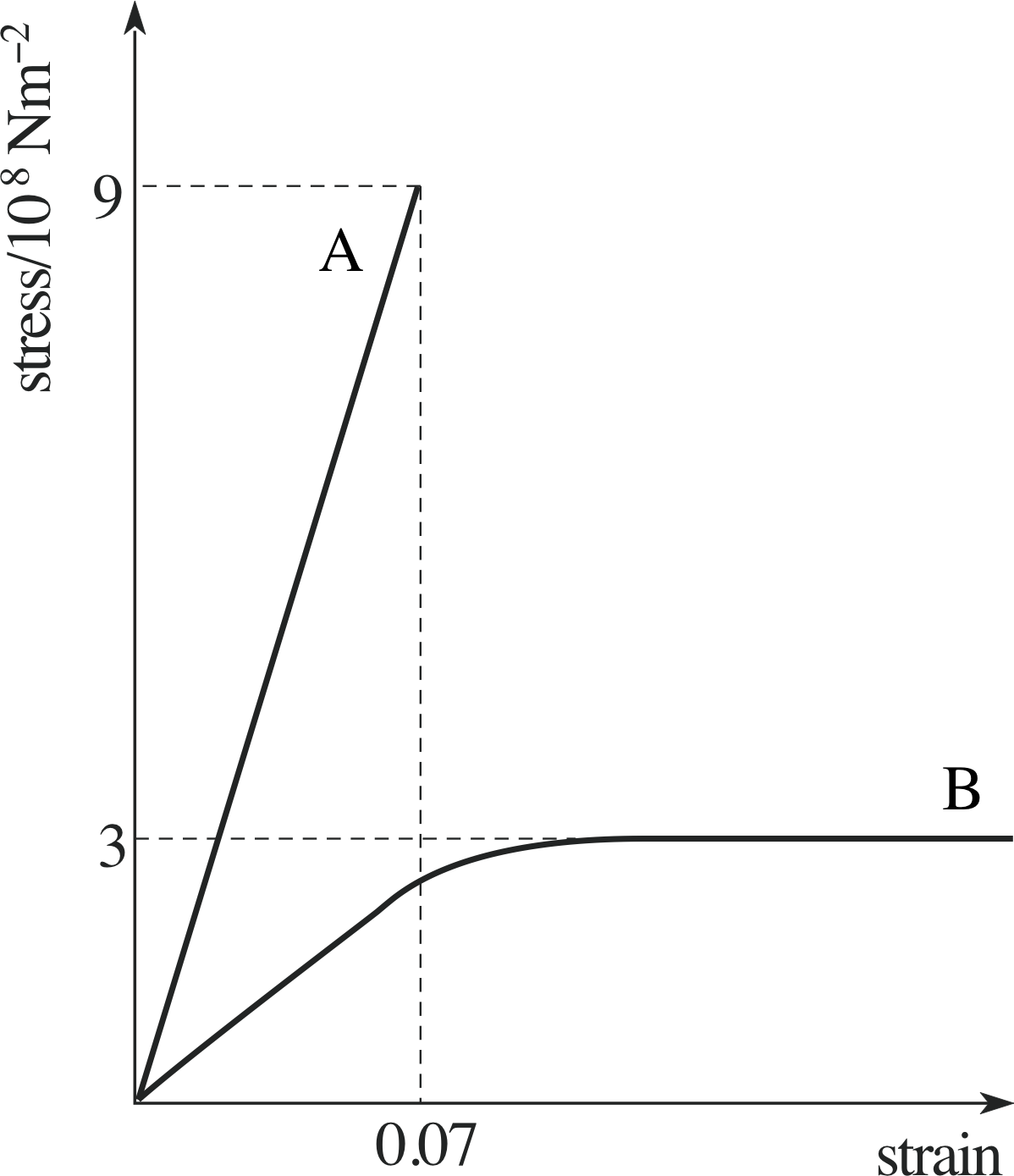
Figure 19 See Answer E2.
Answer E2
See Figure 19. Material A is the most brittle, since it fractures while still in the linear region at comparatively small strains. Since its fracture stress is also the highest, material A is also the strongest.
(Reread Subsections 2.2 and 2.3 if you had difficulty with this question.)
| Material | Y / 1010 N m−2 |
|---|---|
| diamond | 83 |
| steel | 20.0 |
| copper | 11.0 |
| glass (fused quartz) | 7.1 |
| aluminium | 7.0 |
| concrete | 1.7 |
| graphite | 1.0 |
| nylon | 0.36 |
| natural rubber | 0.0007 |
Question E3 (A2)
A structural support element is made of steel and designed so that the maximum shear displacement under the expected shear stress will be 1.0 cm. If the support element were replaced by an identical one made of aluminium, what would be the maximum shear displacement?
Answer E3
The shear displacement and modulus are given by Equations 5 and 6,
shear strain $\varepsilon_{\rm S} = \dfrac{\text{shear between the two surfaces}}{\text{separation between the two surfaces}} = \dfrac{\Delta x}{y}$(Eqn 5)
shear modulus $G = \dfrac{\text{shear stress}}{\text{shear strain}} = \dfrac{\sigma_{\rm S}}{\varepsilon_{\rm S}}$(Eqn 6)
| Material | Y / 1010 N m−2 | G / 1010 N m−2 | K / 1010 N m−2 |
|---|---|---|---|
| aluminium | 7.0 | 2.5 | 7.5 |
| copper | 11.0 | 4.4 | 13.5 |
| steel | 20.0 | 7.5 | 17.0 |
| nylon | 0.36 | 0.12 | 0.59 |
So$\Delta x = \varepsilon_{\rm S}y = \dfrac{\sigma_{\rm S}y}{G}$
If the shear stress and the thickness are the same, then ∆x ∝ 1/G and, using values from Table 2, we can write
$\dfrac{\Delta x_{Al}}{\Delta x_{\rm steel}} = \dfrac{1/G_{\rm steel}}{1/G_{\rm Al}} = \dfrac{G_{\rm steel}}{G_{\rm Al}}$
$\phantom{\dfrac{\Delta x_{Al}}{\Delta x_{\rm steel}} }= \rm \dfrac{7.5\times10^{10}\,Pa}{2.5\times10^{10}\,Pa} = 3.0$
Thus the maximum shear displacement for aluminium would be 3.0 cm.
(Reread Subsection 2.4 if you had difficulty with this question.)
Question E4 (A4)
An experimental apparatus consists of an inner cylinder that is fixed and non–rotating and an outer cylinder that can be rotated with respect to the inner. There is a gap in between the two cylinders, in which a test material such as a solid sleeve can be slipped or liquid poured in, then pressure is applied to the outer cylinder to clamp the test material between the cylinders. Describe the response if the outer cylinder is driven by a motor that can exert a constant force: (a) if the test material is a solid sleeve; (b) if the test material is a liquid.
Answer E4
(a) If the test material doesn’t slip between the inner and outer cylinders, then the motion of the outer cylinder will induce a shear stress in the solid test material. Assuming the applied force isn’t large enough to break the contact with the cylinders, the outer cylinder will stop moving when the induced strain causes a stress within the test material that just balances the applied stress. (If the drive from the motor is rigidly connected then the motor also would be prevented from turning and it could well burn out!)
(b) In the case of the liquid, the motion of the outer cylinder will set up a velocity gradient in the fluid, determined by the applied shear stress and the viscosity of the liquid, and the situation will stabilize with a steady–state rotation of the outer cylinder, with the motor force just balanced by the viscous drag force from the liquid.
(Reread Subsection 4.2 if you had difficulty with this question.)
Question E5 (A5 and A6)
A dam wall designed to hold water in a reservoir is generally thicker at its base than at the top. (a) Explain why this is so. (b) Calculate the force that 1 m2 of the base of the dam wall must withstand if the water level in the reservoir is 40 m. Take atmospheric pressure to be 1.01 × 10⁵ Pa and the density of water as 1.00 × 10³ kg m−3.
Answer E5
(a) The water in the reservoir will develop a hydrostatic pressure which increases with the depth below the surface, being maximum at the bottom. By Pascal’s principle, this will be applied uniformly to the wall of the dam, so that the base of the dam must withstand higher forces than the top.
(b) The additional hydrostatic pressure will be given by ρgh. This must be added to the external atmospheric pressure present at the top. So, at the base:
P = Ph + Pex = ρgh + (1.01 × 10⁵ Pa)
P = (1.00 × 10³ kg m−3 × 9.8 m s−2 × 40.0 m) + (1.01 × 10⁵ Pa)
P = (3.92 × 10⁵ Pa) + (1.01 × 10⁵ Pa) = 4.93 × 10⁵ Pa
This is the pressure at the base, which is equal to the force per unit area.
The force that 1 m2 must withstand is 4.93 × 10⁵ N.
(Reread Subsections 3.1 and 3.2 if you had difficulty with this question.)
Question E6 (A6 and A7)
A hydraulic lift is a form of fluidic amplifier as described in Subsection 3.2. Suppose a lift is designed with a control piston with a radius of 5 cm and a lifting piston with a radius of 30 cm. If the lift is to be able to raise a car of mass 1500 kg, what force must be applied to the control piston?
Answer E6
As developed in Subsection 3.2, Pascal’s principle allows us to equate the pressures on each side of the system and so the relationship between the applied force and the operational force is in the ratio of their piston areas:
$F_{\rm op} = \dfrac{A_{\rm op}}{A_{\rm app}} = \dfrac{\pi(0.30\,{\rm m})^2}{\pi(0.05\,{\rm m})^2}F_{\rm app} = 36F_{\rm app}$
Thus$F_{\rm app} = \dfrac{F_{\rm op}}{36} = \rm \dfrac{1500\,kg\times9.8\,m\,s^{-2}}{36} = 409\,N$
(Reread Subsection 3.2 if you had difficulty with this question.)
Question E7 (A8)
Consider a very simplistic model of a ship, in which we consider it to be a rectangular box made of steel walls 0.10 m thick, with an open top with sides 40 m long, ends 10 m wide, and 10 m high overall. Taking the density of steel to be 7.90 × 10³ kg m−3, where is the water line if the ship is floating in sea water of density 1.03 × 10³ kg m−3?
Answer E7
The mass of this simplistic ship is given by the volume of the walls times the density of steel. The total area of the walls and base is given by
area = (3 × 40 m × 10 m) + (2 × 10 m × 10 m) = 1.4 × 10³ m2
This is then multiplied by the wall thickness and the density to yield the mass:
M = 1.4 × 10³ m2 × 0.10 m × 7.90 × 103 kg m−3 = 1.1 × 10⁶ kg
The weight of the ship is then
Mg = 1.1 × 106 kg × 9.81 m s−2 = 1.08 × 10⁷ N
which is the required buoyancy force.
By Archimedes’ principle, this must be equal to the weight of the displaced sea water. Assuming the ship, of base area Abase, displaces water to a depth d, the displaced volume will be given by Vd = Abased and the buoyancy force will be FB = ρgVd.
So the depth submerged is
$d = \dfrac{Mg}{\rho gA_{\rm base}} = \rm \dfrac{1.08\times10^7\,N}{1.03\times10^3\,kg\,m^{-3}\times9.8\,m\,s\,^{-2}\times40\,m^2} = 2.67\,m$
(Reread Subsection 3.3 if you had difficulty with this question.)
Question E8 (A9)
Suppose you had a block sliding on a surface of the same material. Assuming that the conditions of strength, elasticity, and cleanliness were the same, if you wanted to minimize the friction, would you make the surfaces as rough or as smooth as possible? Explain why.
Answer E8
If all other properties of the interface were the same, then to minimize friction, you would want to make the surface rough (at least microscopically), because the largest source of friction is the adhesion force from the actual microscopic contact areas. Making the surface smooth would maximize this contact area, and hence make the friction large.
(Reread Subsection 4.1 if you had difficulty with this question.)
| Liquid | η/10−3 Pa s |
|---|---|
| glycerine | 830 |
| mercury | 1.58 |
| olive oil | 84 |
| water | 1.01 |
Figure 12 A fluid is contained between two parallel plates in uniform relative motion. The rectangles indicate the velocity profile of the fluid with respect to the bottom plate.
Question E9 (A10)
An experiment to measure viscosity (Figure 12) has a plate separation of 2 mm. It is found that a shear stress of 0.20 N m−2 produces a relative velocity of 5 mm s−1.
From Table 3, identify the sample.
| Liquid | η/10−3 Pa s |
|---|---|
| glycerine | 830 |
| mercury | 1.58 |
| olive oil | 84 |
| water | 1.01 |
Answer E9
For this, we need to use Equation 15,
$\sigma_x = \eta\dfrac{\Delta\upsilon_x}{\Delta y}$(Eqn 15)
relating the shear stress to the velocity gradient.
So we have:
$\eta = \dfrac{\Delta y\sigma_x}{\Delta\upsilon_x} = \rm \dfrac{2.0\,mm\times0.20\,N\,m^{-2}}{5.0\,mm\,s^{-1}} = 8.0\times10^{-2}\,Pa\,s$
Consulting Table 3, the closest value identifies the sample as olive oil.
(Reread Subsection 4.2 if you had difficulty with this question.)
| Liquid | η/10−3 Pa s |
|---|---|
| glycerine | 830 |
| mercury | 1.58 |
| olive oil | 84 |
| water | 1.01 |
Question E10 (A11)
A steel ball bearing is falling in a tank of glycerine. Taking the diameter of the ball bearing to be 4.0 mm, the density of the bearing to be 8.0 × 10³ kg m−3, the density of the glycerine to be 1.3 × 1031 kg m−3 and the viscosity of the glycerine from Table 3, use Stokes’ law to calculate the terminal speed of the ball bearing.
Answer E10
We assume that the ball bearing is spherical, and use Equation 17,
terminal velocity $\upsilon_{\rm t} = \dfrac{\left(\rho_{\rm sphere} - \rho_{\rm fluid}\right)Vg}{6\pi a\eta}$(Eqn 17)
and Answer T11:
$\upsilon_{\rm t} = \dfrac{\left(\rho_{\rm sphere} - \rho_{\rm fluid}\right)Vg}{6\pi a\eta} = \dfrac{2a^2g}{9\eta}\left(\rho_{\rm sphere} - \rho_{\rm fluid}\right)$
Now
ρsphere − ρfluid = (8.0 − 1.3) × 103 kg m−3 = 6.7 × 10³ kg m−3
so$\upsilon_{\rm t} = \rm \dfrac{2\times(2.0\times10^{-3}\,m)^2\times9.8\,m\,s^{-2}\times6.7\times10^3kg\,m^{-3}}{9\times830\times10^{-3}\,Pa\,s} = 70\,mm\,s^{-1}$
(Reread Subsection 4.3 if you had difficulty with this question.)
Question E11 (A12)
Two bubbles with radii R1 and R2 are connected by a small tube. Initially, a valve in the middle of the tube is closed, so that the bubbles are isolated from each other. Describe what happens when the valve is opened, assuming R2 > R1, and the surface tension is the same for each bulb. Explain your reasoning.
Answer E11
To understand what happens when the valve is opened, we have to consider the internal pressures in the two bubbles before the valve is opened. Using Equation 20,
excess pressure $P - P_{\rm ex} = \dfrac{16\pi\gamma R\Delta R}{4\pi R^2\Delta R} = \dfrac{4\gamma}{R}$(Eqn 20)
the pressure excess in either bubble will be given by:
$(P - P_{\rm ex}) = \dfrac{4\gamma}{R}$
The external pressure will be the same for both bubbles and so we see that the internal pressure is higher in the smaller bubble (R = R1). When the connecting tap is opened, air will flow from the smaller to the larger bubble until the only trace of the smaller bubble is a film across the end of the tube (which will actually have the same radius of curvature as the final state of the larger bubble).
(Reread Subsection 4.4 if you had difficulty with this question.)
Question E12 (A13)
A glass capillary tube of diameter 1 mm is inserted vertically into a dish of mercury. Describe what happens and calculate the final level of the mercury within the capillary. Take the angle of contact between glass and mercury to be 140°, and the density of mercury as 1.35 × 10⁴ kg m−3.
Answer E12
| Liquid | γ/10−3 N m−1 |
|---|---|
| glycerine | 63.1 |
| mercury | 475 |
| olive oil | 32.0 |
| water | 72.8 |
Since the contact angle is greater than 90°, the level of the mercury will be depressed in the capillary tube. Equation 21,
$h = \dfrac{2\pi r\gamma\cos\theta}{\pi r^2\rho g} = \dfrac{2\gamma\cos\theta}{r\rho g}$(Eqn 21)
with γ from Table 4 gives:
$h = \rm \dfrac{2\times475\times10^{-3}\,N\,m^{-1}\times\cos40°}{5\times10^{-4}\,m\times1.35\times10^4\,kg\,m^{-3}\times9.8\,m\,s^{-2}} = -10.99\,mm$
So the mercury will be depressed by about 11 mm.
(Reread Subsection 4.4 if you had difficulty with this question.)
Study comment This is the final Exit test question. When you have completed the Exit test go back and try the Subsection 1.2Fast track questions if you have not already done so.
If you have completed both the Fast track questions and the Exit test, then you have finished the module and may leave it here.
Study comment Having seen the Fast track questions you may feel that it would be wiser to follow the normal route through the module and to proceed directly to the following Ready to study? section.
Alternatively, you may still be sufficiently comfortable with the material covered by the module to proceed directly to the Section 5Closing items.