PHYS 8.2: Atomic spectra and the hydrogen atom |
PPLATO @ | |||||
PPLATO / FLAP (Flexible Learning Approach To Physics) |
||||||
|
1 Opening items
1.1 Module introduction
The hundred or so different kinds of atom are the basic building blocks of all of the familiar forms of matter. A typical atom has a diameter of about 10−10 m and consists of one or more negatively charged electrons moving under the electrical attraction of a small, dense, positively charged nucleus. The centrally located nucleus has a diameter of about 10−14 m and occupies less than one trillionth (10−12) of an atom’s volume, yet it contains more than 99.9% of its mass.
The presence of a nucleus at the heart of every atom was proposed in 1911 by Ernest_RutherfordErnest (later Lord) Rutherford (1871–1937) on the basis of experiments in which α–particles (i.e. the nuclei of helium atoms) were observed to rebound or scatter from gold atoms in thin metal foils. The concept of the atomic nucleus quickly gained widespread acceptance, but some of Rutherford’s other ideas about the structure of atoms did not fare so well. In particular, his suggestion that each atom was like a miniature Solar System, in which the electrical force held the electrons in orbit around the nucleus in much the same way that gravitational forces bind the planets to the Sun, was soon shown to be inconsistent with the laws of physics as they were then known. The overthrow of this ‘planetary model’ of the atom – still the most advanced model that most non–physicists meet – raised the problem of understanding the internal structure of atoms to one of crucial importance and opened the way for the development of other models of atomic structure that called on ideas from the new field of quantum physics.
This module describes the first important ‘quantum model’ of the atom and some of the evidence that supported it. Under appropriate conditions, atoms can emit or absorb light; Section 2 describes the way in which the light emitted or absorbed by any particular type of atom can be used to characterize that atom and provide insight into its internal structure. It introduces the concept of an atomic spectrum and defines some of the main kinds of spectra that can be observed. Section 3 concentrates on the simplest atomic spectrum – that of the hydrogen atom. With just a single electron bound to its nucleus, hydrogen is the simplest of atoms and represents a natural starting point for efforts to understand the structure of atoms in general. Section 4 provides a detailed account of the model of the hydrogen atom put forward in 1913 by the Danish physicist Niels Bohr (1885–1962). Although now known to be fundamentally flawed, just like Rutherford’s model, Bohr’s model gives real insights into atomic structure and is an excellent starting point from which to discuss more modern theories of the atom. Bohr’s theory is of great historical importance since it prepared the way for Werner Heisenberg (1901–1976), Erwin Schrödinger (1887–1961) and others who set down the basic principles of our current quantum theory of atomic structure in the mid-1920s.
Study comment Having read the introduction you may feel that you are already familiar with the material covered by this module and that you do not need to study it. If so, try the following Fast track questions. If not, proceed directly to the Subsection 1.3Ready to study? Subsection.
1.2 Fast track questions
Study comment Can you answer the following Fast track questions? If you answer the questions successfully you need only glance through the module before looking at the Subsection 5.1Module summary and the Subsection 5.2Achievements. If you are sure that you can meet each of these achievements, try the Subsection 5.3Exit test. If you have difficulty with only one or two of the questions you should follow the guidance given in the answers and read the relevant parts of the module. However, if you have difficulty with more than two of the Exit questions you are strongly advised to study the whole module.
Question F1
Explain how and why the absorption spectrum of an element differs from its emission spectrum, as observed in the laboratory. Briefly describe an experimental arrangement that will allow the absorption spectrum of a gas to be observed.
Answer F1
At all reasonable laboratory temperatures there are very few atoms excited out of the ground state. Under these conditions it is impossible to observe absorption from any state other than the ground state since atoms are only available in this state. In emission, where atoms start from many possible excited states, more transitions can be involved. The emission spectrum thus contains far more lines than the absorption spectrum. The absorption spectrum may be studied by passing white light through a vapour of atoms and then using a grating spectrometer to observe the dark absorption lines which cross the continuous spectrum of white light.
Question F2
Given the following expression for the energy levels of atomic hydrogen
$E_n = -\left(\dfrac{\mu_{\rm e}e^4}{8\varepsilon_0^2h^2}\right)\left(\dfrac{1}{n^2}\right) = -\left(\dfrac{13.6}{n^2}\right)\,{\rm eV}$
evaluate the atom’s ionization energy and the wavelength of the first (lowest frequency) line in the Lyman series.
Answer F2
The ionization level E3 has zero energy, corresponding to n → ∞, and the ground state has an energy E1 = −13.6 eV. The ionization energy is the energy needed to take the electron from the ground level to the ionization level. This is therefore 13.6 eV.
The first line in the Lyman series corresponds to a transition between levels n = 2 and n = 1. The energy difference is
$E_2-E_1 = \rm 13.61\,\left(\dfrac11-\dfrac14\right)\,eV = 10.2\,eV$
To calculate the wavelength we need to use SI units for energy and to substitute values into Equation 6,
$\lambda = \dfrac{hc}{\lvert\,E_{\rm i}-E_{\rm f}\,\rvert}$(Eqn 6)
$\lambda_{2\to1} = \dfrac{hc}{E_2-E_1} = \rm \dfrac{6.63\times10^{-34}\times3.00\times10^8}{10.2\times1.60\times10^{-19}}\,m = 122\,nm$
1.3 Ready to study?
Study comment To study this module you will need to understand the following terms: absolute temperature, angular momentum, angular frequency, atom, Boltzmann’s constant, centripetal force, circular motion, Coulomb’s law, diffraction grating, dispersion, electric potential energy, electromagnetic radiation, electromagnetic spectrum (including ultraviolet_radiationultraviolet and infrared_radiationinfrared), electronvolt, conservation_of_energyenergy conservation, force, frequency, grating_relationthe grating relation (nλ = d sin θn), kinetic energy, molecule, momentum, conservation_of_momentummomentum conservation, Newton’s laws of motion, orders of diffraction, wavelength. In addition, some familiarity with the use of algebrabasic algebra, exponential_functionexponentials, graph_sketchinggraph plotting, logarithms and trigonometric functions will be assumed.
If you are uncertain about any of these terms, review them now by reference to the Glossary, which will also indicate where in FLAP they are developed. The following Ready to study questions will allow you to establish whether you need to review some of the topics before embarking on this module.
Question R1
A beam of light of wavelength λ = 541 nm is normally incident on a diffraction grating which has 600 lines mm−1. Determine the angle θ2 at which the second order diffracted beam is seen.
Answer R1
The grating relation must be used here:
nλ = d sin θn
with d = (1/600) mm = 1.67 × 10⁻⁶ m
In order_of_diffractionsecond order we have n = 2 and so:
$\sin\theta_n = \dfrac{2\lambda}{d} = \rm \dfrac{2\times541\times10^{-9}}{1.67\times10^{-6}} = 0.648$
∴θ2 = arcsin 0.648 = 40.4°
(If you are unsure about any of these terms, consult the Glossary.)
Question R2
An electron is emitted from a heated metal surface and is accelerated through a potential difference of +5 V. Determine the potential energy change and the kinetic energy change for the electron; express your answer both in electronvolts (eV) and in basic SI units.
Answer R2
The electron gains 5 eV of kinetic energy and loses 5 eV of potential energy as it rises through the 5 V potential difference. This comes directly from the definition of the electronvolt.
Since 1 eV = 1.60 × 10⁻¹⁹ J the equivalent energy change in SI units is 5 eV = 8.00 × 10⁻¹⁹ J.
(If you are unsure about any of these terms, consult the Glossary.)
Question R3
Describe the distinction between an atom and a molecule.
Answer R3
An atom is the smallest part of an element having the chemical identity of that element; a molecule consists of two or more atoms of the same or different elements bound together in characteristic units. Molecules are the smallest part of a material having the same chemical identity as the material as a whole.
(If you are unsure about any of these terms, consult the Glossary.)
Comment While the distinction between atom and molecule given in Answer R3 is generally made, there are occasions where the term ‘molecule’ is used to include ‘atom’ as a special case. In this module we will use the distinction given in Answer R3.
Question R4
Visible light constitutes one small part of the electromagnetic spectrum. Write down an expression which shows how the wavelengths and frequencies of light relate to the speed of light in a vacuum.
Answer R4
The electromagnetic spectrum consists of all electromagnetic waves which are able to travel through a vacuum with a common velocity of c = 3 × 10⁸ m s−1.
For each of these electromagnetic waves the wavelengths and frequencies are related through c = f λ.
For visible light the fairly narrow range is from red, at λ ≈ 7.0 × 10⁻⁷ m or 700 nm (f = 4.3 × 10¹⁴ Hz) to violet at λ ≈ 4.0 × 10⁻⁷ m or 400 nm (f = 7.5 × 10¹⁴ Hz).
(If you are unsure about any of these terms, consult the Glossary.)
Question R5
A constant force F acts on a particle of mass m. Write down an expression for the acceleration a of the particle.
Answer R5
Acceleration a = F/m from Newton’s second law of motion.
(If you are unsure about any of these terms, consult the Glossary.)
Question R6
A particle of mass m is moving with speed υ along a circular path of radius r and has an angular frequency ω. Write down expressions for:
(a) the magnitude of the momentum of the particle;
(b) the kinetic energy of the particle;
(c) the magnitude and direction of the centripetal force acting on the particle;
(d) the magnitude of the angular momentum of the particle about the origin.
Answer R6
(a) The magnitude of the momentum p = mυ = mrω
(b) The kinetic energy is Ekin = mυ2/2 = mr2ω2/2
(c) The centripetal force is of magnitude Fr = mυ2/r = mrω2 and is directed towards the centre of the orbit.
(d) The electron’s angular momentum (L = r × p) has a magnitude of L = rp sin θ where θ is the angle between r and p. In this case θ is 90° so sin θ = 1; the magnitude of L is L = rp = mυr.
(If you are unsure about any of these terms, consult the Glossary.)
Question R7
Two electric charges, each of 1 μC, are 10 mm apart. Write down Coulomb’s law and calculate the magnitude of the force acting on each of the charges, given that the permittivity of free space is ε0 = 8.85 × 10⁻¹² C2N−1 m−2.
Answer R7
Coulomb’s law gives the magnitude of the force between charges q1 and q2 when separated by a distance r as
$F = \dfrac{q_1q_2}{4\pi\varepsilon_0r^2}$
where ε0 = 8.85 × 10⁻¹² C2 N−1 m−2 is the permittivity of free space
If we substitute numerical values we find that:
$F = \rm \dfrac{10^{-6}\times10^{-6}}{4\pi\times8.85\times10^{-12}(10^{-2})^2}\,N = 89.9\,N$
(If you are unsure about any of these terms, consult the Glossary.)
2 The production of atomic spectra
2.1 Characteristic emission spectra
When chemical substances are vaporized in a flame they emit light. This light typically covers a range of wavelengths and, when appropriately dispersed, so that different wavelengths travel in different directions, it reveals what is known as the emission spectrum of the substance. The spectrum emitted by each of the chemical elements is of particular interest and is known as the characteristic emission spectrum of the element. Spectroscopy is the branch of science that is concerned with the study of spectra; it originated in the early nineteenth century and had developed considerably by the end of the 1850s.
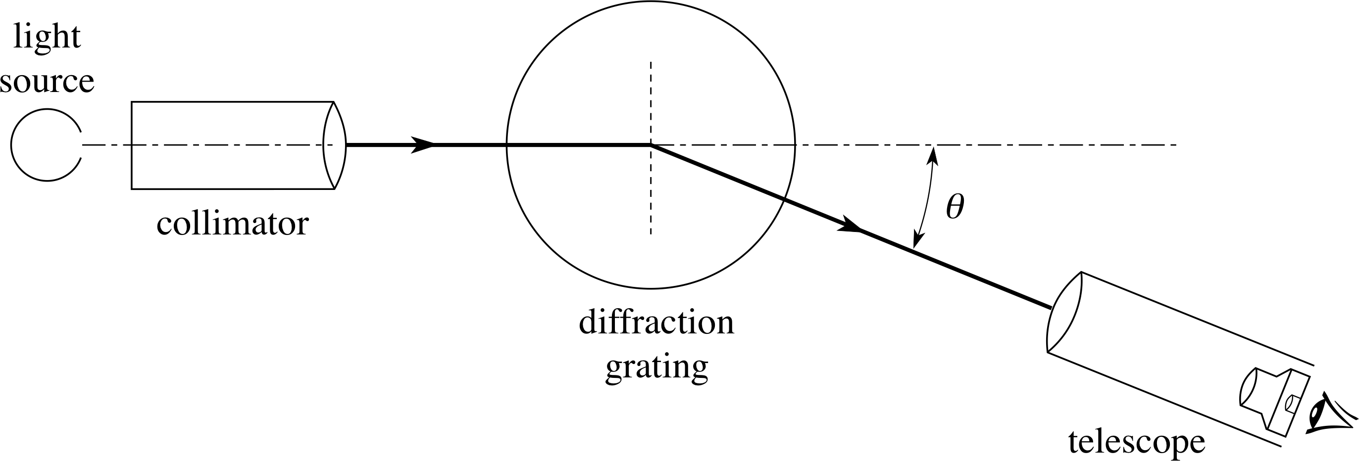
Figure 1 Experimental arrangement for the observation of an emission spectrum. The general requirements are a source of the light to be studied, a means of splitting (dispersing) the light into its constituent wavelengths and a detector. The source of light may be a flame, a hot body or a purpose–made spectral lamp.
A simple experimental arrangement for the observation of an emission spectrum is shown in Figure 1.
The instrument used to measure wavelength is a spectrometer.
A spectrometer usually contains a collimator, which produces a parallel beam of light from a slit, a dispersion device (usually a diffraction grating or a triangular glass prism) and a telescope. As the beam of light from the collimator passes through the dispersion device the constituent wavelengths in the beam to travel in different directions, so they appear at different angles when viewed through the telescope.
If the dispersion device is a diffraction grating, light of a given wavelength λ will be observed at particular angles θ1, θ2, θ3, etc. as given by the grating relation nλ = d sin θn, where n is the order of diffraction and d is the grating spacing (i.e. the distance between adjacent slits on the grating).
This simple method of determining wavelengths can be used to analyse the yellow light emitted by sodium when it is heated in a flame.
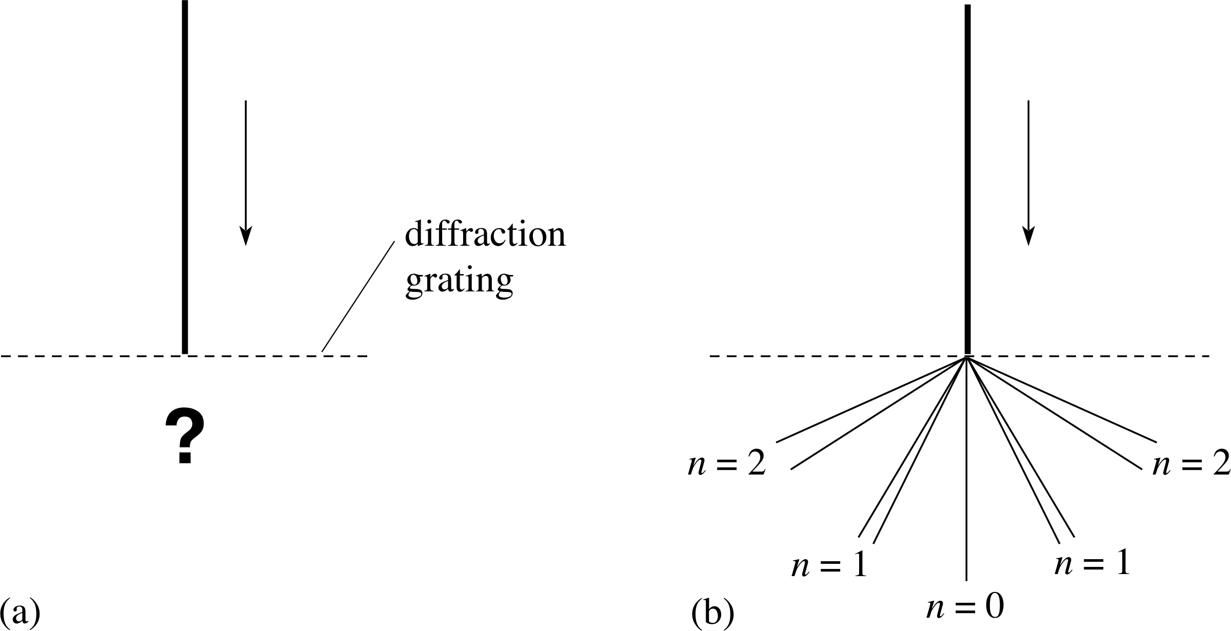
Figure 2 (a) What happens when a parallel beam of yellow sodium light is shone on to a diffraction grating? When the light emerges from the grating it does not produce broad bands of light in each order, corresponding to the full range of yellow light (580 nm to 600 nm), but rather lines at definite angles corresponding to particular wavelengths as in (b). In fact it is found that the yellow sodium light consists of two separate wavelengths at 589.0 nm and 589.6 nm and the spectrum appears as pairs of narrowly separated yellow lines – a doublet – in each order of diffraction (except n = 0), as is shown in (b). In each of the four doublet images the separation has been exaggerated.
Consider what happens when a collimated beam of this yellow light falls on a diffraction grating as shown in Figure 2a. If this yellow light consisted of all wavelengths in the yellow part (580–1600 nm) of the visible electromagnetic spectrum, the light would produce several separated but continuous bands on either side of the straight–through beam with each band corresponding to a different order of diffraction for light in this wavelength range. But this does not happen. Instead, the yellow light is diffracted only at certain, definite angles. This implies that the yellow sodium light contains only certain narrowly defined ranges of wavelength – so narrow that they appear as ‘lines’ rather than ‘bands’ when viewed with the spectrometer. Such lines, seen in an emission spectrum, are known as emission lines.
The sodium light consists mainly of two emission lines, one at 589.0 nm and the other, very nearby, at 589.6 nm. Both are in the yellow part of the spectrum, so what is seen through the spectrometer is a pair of narrowly separated yellow lines – a doublet – in each order of diffraction (except n = 0), as is shown in Figure 2b.
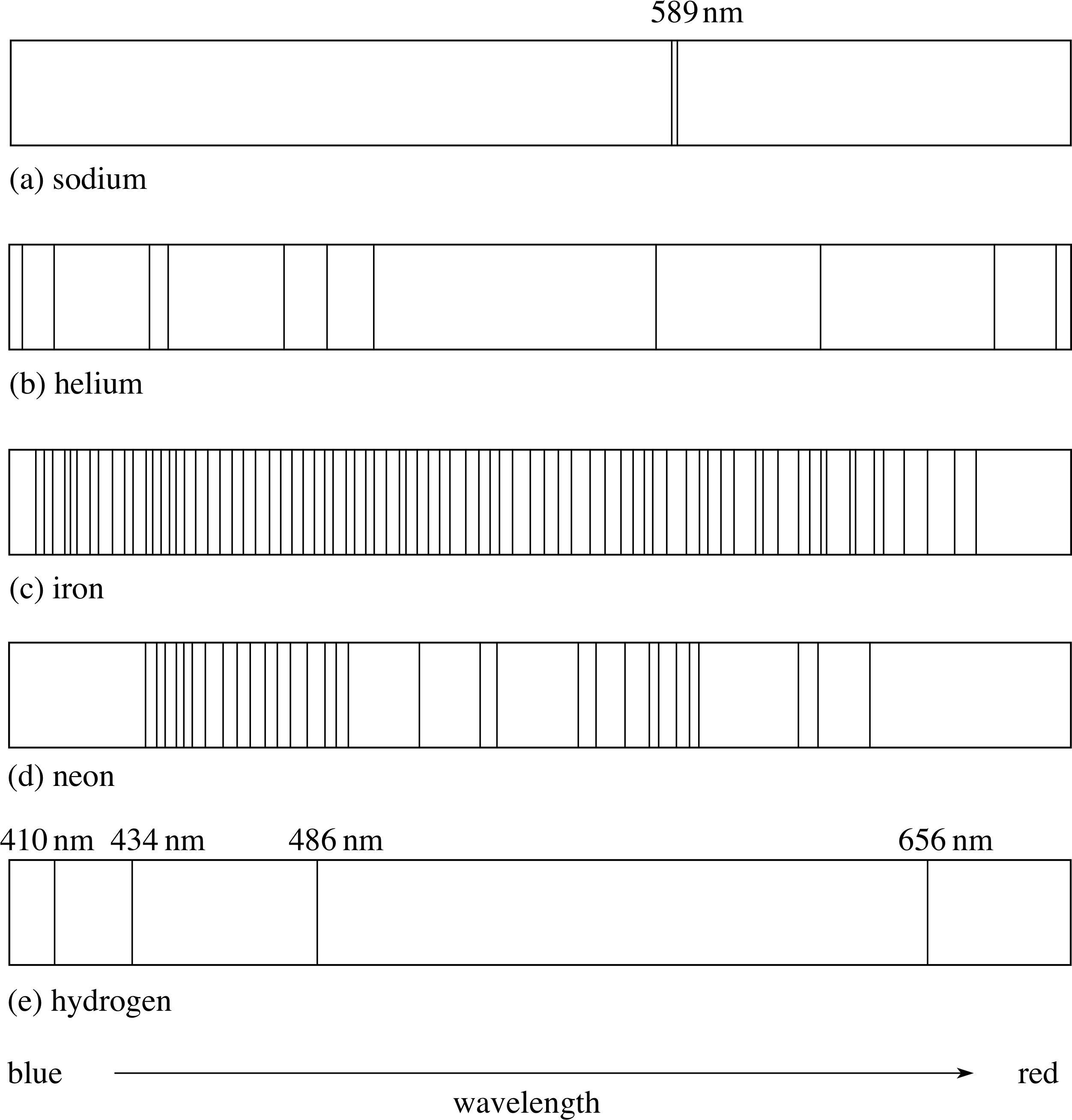
Figure 3 Schematic diagram illustrating the characteristic emission spectra or line spectra of (a) sodium, (b) helium, (c) iron, (d) neon and (e) hydrogen. Only the brightest spectral lines have been shown, especially in the case of sodium.
Each element has its own characteristic emission spectrum, that is, its own individual pattern of emission lines. Sometimes this pattern is called the emission line spectrum of the element. The characteristic emission spectra, or line spectra, of various elements are shown schematically in Figure 3. i
The fact that each element has its own characteristic line spectrum is the basis of an important technique of chemical analysis. If the line spectrum of an element is identified within the emission spectrum of a chemical sample, it can be concluded that the sample contains that particular element. This principle is also used in astrophysics to identify the elements present in the emitting regions of astronomical bodies.
Direct heating is not the most common method used for the production of line spectra in the laboratory. The most popular method, which is also used in spectral lamps such as street lamps and advertising signs, is to pass a beam of electrons through a gas or vapour. If the kinetic energy of each electron in the beam is above a few electronvolts, collisions with atoms in the gas result in the transfer of energy to the atoms. The energy is then re–emitted by the atoms, producing the line spectrum.
This method is used where the material is either gaseous at room temperature or can be vaporized by moderate heating. Line spectra from materials that are difficult to vaporize, such as iron or tungsten, can be produced by placing them on electrodes across which there is an electric discharge.
2.2 Continuous emission spectra; the black–body spectrum
Although the line spectrum of a vaporized element can be produced as described above, if the element remains solid or liquid, even when heated to a high temperature, the emitted spectrum does not generally consist of characteristic emission lines. Rather, all possible wavelengths within a wide continuous range are present. Because of its unbroken nature, such a spectrum is called a continuous_spectrumcontinuous emission spectrum. Ordinary white light provides one example of this, since it can be dispersed by a diffraction grating or a prism into all the colours of the rainbow.
The experimental arrangement shown in Figure 1 can be used to study this when the light source is a hot body, such as the tungsten filament of an electric light bulb.
When the spectra from hot bodies are examined and the power emitted per unit area of the source per unit wavelength range (often referred to as spectral brightness) is plotted as a function of wavelength, it is found that the graphs all approximate, to a greater or lesser extent, the same idealized shape. This idealized shape is achieved most closely when the surface of the emitter is black; a black surface absorbs all of the radiation which falls on to it and reflects none. For this reason, an idealized emitter is known as a black body and the idealized spectrum it produces is known as a black–body spectrum. i
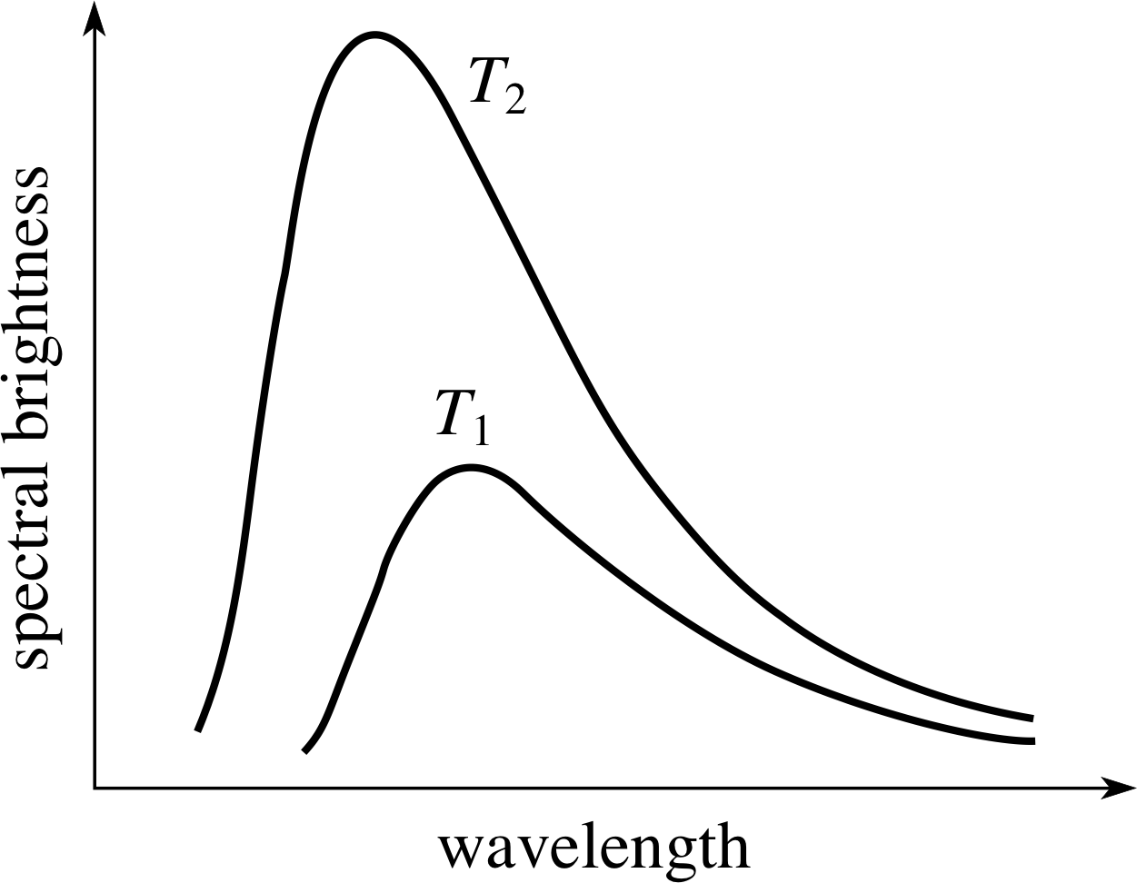
Figure 4 Black–body spectra from an idealized hot body at two different temperatures (T2 > T1).
A very close approximation to a black body can be made by cutting a small hole in a hollow body. The radiation coming from the hole when the body is hot approximates very closely to a black–body spectrum. Since the hole absorbs any radiation falling on to it from outside the body, the hole can be considered to be perfectly black. The shape of the black–body spectrum, the wave–length for peak emission, and the total radiated power per unit area of the surface are all determined entirely by the temperature of the body. i Examples of black–body spectra, from a body at two different temperatures, are shown in Figure 4.
Figure 4 shows that the hotter the black body the shorter the wavelength for peak emission – it moves from the red to the blue end of the spectrum as the temperature increases. Even though non–black bodies generally emit less power per unit area in a given wavelength interval than a true black body, this general shift in the peak emission wavelength with temperature is familiar to anyone who has observed an electric fire heating up or a tungsten filament light bulb as the current through it is controlled by a dimmer switch. The observed spectrum from the Sun and other stars conforms quite closely to that of a black body, and in astrophysics the surface temperature of a star is often estimated from its colour. Red stars are relatively cool and blue stars are very hot; our own yellow star, the Sun, is intermediate between these extremes and has a surface temperature of around 6 000 K.
2.3 Absorption spectra
When a vapour of atoms or molecules is illuminated by a source having a continuous spectrum (e.g. white light), the atoms or molecules selectively absorb certain wavelengths. The pattern of absorbed wavelengths is known as the absorption spectrum of the atoms or molecules. Often the absorption spectrum consists of a set of characteristic absorption lines and the spectrum is then often referred to as the absorption line spectrum. The observed spectrum therefore consists of the original continuous spectrum of the source, interrupted by dark lines which are the characteristic absorption lines of the atoms or molecules in the vapour.
The experimental arrangement to study an absorption spectrum is very similar to that shown in Figure 1. However, to observe an absorption spectrum, an absorption cell containing a gas or vapour of the atoms to be studied is placed between the collimator and diffraction grating. Since atoms only absorb their own characteristic wavelengths, these precise wavelengths must be provided in order to study the absorption. In practice, this usually requires either a source containing identical atoms or one which provides a continuous spectrum.
If the wavelengths of the lines seen in absorption are measured it is found that these same wavelengths are also seen in the emission spectrum of the element. However, the emission spectrum includes many additional lines which are not normally seen in absorption. We shall consider the reason for this in Section 5.
2.4 Summary of Section 2
This section has introduced emission spectra and absorption spectra. Atoms of each element are capable of emitting or absorbing light. In emission an atom loses energy which is carried away by the light that it emits and in absorption an atom gains energy from the incoming light which it absorbs. Only a restricted number of definite wavelengths are involved in the emission and absorption from atoms of any particular element. These particular wavelengths, or spectral_lineslines, are specific to atoms of that particular element and the set of these lines constitutes the characteristic emission spectrum of that element. Once the characteristic spectrum of an element is known the observed spectral lines from an unknown source are usually sufficient to indicate the presence or absence of that element in the unknown source.
In addition to the characteristic emission and absorption lines from each element it is possible to observe light emission from hot bodies. The continuous spectrum from a hot body consists of a continuous range of wavelengths. An idealized hot–body emitter is called a black body and the associated continuous spectrum is known as a black–body spectrum. A black body has a surface which is totally absorbing of any radiation which falls on to it; real emitters approximate this to some extent.
For black–body sources, the variation in relative brightness with wavelength, the wavelength for peak brightness and the total radiated power per unit area of the surface all depend on the temperature alone; as the temperature is increased, the peak emission shifts to shorter wavelengths and the total radiated power increases.
The observation of an absorption spectrum usually requires the vapour or gas to be illuminated by a continuous spectrum; the absorption lines then appear as dark lines against the bright background of the continuous spectrum.
Question T1
Explain in your own words how the absorption and emission spectra of an atom can be observed and describe how their appearance differs.
Answer T1
Observation of the emission spectrum requires a vapour lamp, probably with electron beam collisions to raise the energy of the atoms, and a spectrometer with a diffraction grating to separate the various characteristic lines. The spectrum appears as bright lines on a dark background.
The absorption spectrum is observed by using a white light source and passing the light from this through the vapour and then into a spectrometer. The spectrum appears as dark lines on the bright background of the continuous spectrum from the source. The absorption spectrum will contain fewer lines than the emission spectrum.
Figure 4 Black–body spectra from an idealized hot body at two different temperatures (T2 > T1).
Question T2
Give, in your own words, three major differences between the two black–body spectra shown in Figure 4.
Answer T2
First, the wavelength for maximum emission becomes smaller (i.e. peak of curve shifts towards the blue) as the temperature increases.
Second, the total energy emitted over all wavelengths (proportional to the area under the curve) increases with rising temperature.
Third, the spread in wavelengths (i.e. the width of the curve) increases with rising temperature.
By 1860, spectroscopists had determined the characteristic emission and absorption spectra of many elements. That was a significant achievement, but the really difficult problem was to interpret those spectra. What could be concluded about atoms from their patterns of spectral lines?
So far, we have mentioned the spectra of complicated elements such as sodium, helium, iron and neon. But what about the spectrum of hydrogen, the element that contains the lightest (and simplest?) atoms of all? The spectrum of atomic hydrogen turns out to be the key to the quantitative understanding of all spectra; you have seen part of this spectrum already, in Figure 3e.
3 The emission spectrum of atomic hydrogen

Figure 3e Schematic diagram illustrating the characteristic emission spectra or line spectra of hydrogen. Only the brightest spectral lines have been shown.
The interpretation of spectra from multi–electron atoms is extremely complicated, even by today’s standards. The understanding of atomic spectra must begin with the simplest atom of all – hydrogen. Hydrogen does not occur naturally as single atoms but rather as diatomic molecules, H2. i The spectrum of molecular hydrogen is similar to, but more complicated than, that of atomic hydrogen. To observe the spectrum of atomic hydrogen requires the hydrogen molecules to be broken into individual atoms, a process known as dissociation. Fortunately the conditions existing within a spectral lamp, as described in Section 2, cause dissociation of many of the H2 molecules and so the atomic hydrogen spectrum is quite easy to produce. It consists of a set of characteristic lines in the visible part of the electromagnetic spectrum, one set in the ultraviolet region and several sets in the infrared region. The visible spectrum, shown in Figure 3e, was well known by the latter part of the nineteenth century, but observations of the ultraviolet and infrared lines required more sophisticated spectrometers and therefore came later.
3.1 The visible spectrum of atomic hydrogen; Balmer’s formula
In 1885 Johann Balmer (1825–1898), a Swiss mathematics teacher, found an interesting mathematical relationship which described the wavelengths of the known visible lines in the spectrum of atomic hydrogen. The observed lines have wavelengths 656.21 nm (red), 486.07 nm (blue/green), 434.01 nm (blue/violet) and 410.12 nm (violet). i
Balmer discovered that these wavelengths were given to an extraordinary accuracy by the expression
$\lambda = 364. 56\left(\dfrac{n^2}{n^2-4}\right)$ nanometres (Balmer’s formula)(1)
This expression has become known as Balmer’s formula and the spectral lines whose wavelengths fit this formula became known as the Balmer series. The number n is an integer (a whole number) with values 3 (red line), 4 (blue/green line), 5 (blue/violet line) and 6 (violet line). i The precision of this fit is remarkable and it was surmised that there must be some fundamental physical reason for this. In particular, the variation of wavelength with n2 and the appearance of the integer 4 (= 22) raised interesting questions.
Question T3
Calculate the discrepancies in the wavelengths for the four visible lines in the spectrum of atomic hydrogen, as observed and as predicted by Balmer’s formula using the values of n given above.
Answer T3
The observed lines have wavelengths 656.21 nm (red), 486.07 nm (blue/green), 434.01 nm (blue/violet) and 410.12 nm (violet).
Balmer’s formula is
$\lambda = 364. 56\left(\dfrac{n^2}{n^2-4}\right)\,{\rm nanometres}$(Eqn 1)
so we need to substitute the values of n = 3, 4, 5 and 6 to test the agreement. If we calculate the discrepancies ∆ as ∆ = (λBalmer − λobserved):
For n = 3, $\lambda = 364. 56\left(\dfrac{9}{9-4}\right)\,{\rm nm} = 656.21\,{\rm nm}$
with ∆ = 0.00 nm
For n = 4, $\lambda = 364. 56\left(\dfrac{16}{16-4}\right)\,{\rm nm} = 486.08\,{\rm nm}$
with ∆ = 0.01 nm
For n = 5, $\lambda = 364. 56\left(\dfrac{25}{25-4}\right)\,{\rm nm} = 434.00\,{\rm nm}$
with ∆ = −0.01 nm
For n = 6, $\lambda = 364. 56\left(\dfrac{36}{36-4}\right)\,{\rm nm} = 410.13\,{\rm nm}$
with ∆ = 0.01 nm
The agreement between these values and the measured ones is impressive.
The significance of Balmer’s formula increased following experimental confirmation of his prediction of new lines, having shorter wavelengths, and corresponding to larger values of n. All these fall in the visible or near ultraviolet region of the electromagnetic spectrum.
From Figure 3e and from your calculations in Question T3 it should be apparent that as we move to shorter wavelengths, the successive members of the Balmer series become closer and closer together in wavelength.
The line wavelengths are converging to the Balmer series limit, which corresponds to the shortest possible wavelength for a member of the Balmer series. i
✦ What value of n in Balmer’s formula corresponds to the Balmer series limit? Use this to find the series limit.
✧ From Balmer’s formula,
$\lambda = 364.56\left(\dfrac{n^2}{n^2-4}\right)\,{\rm nanometres}$(Eqn 1)
we can see that as n becomes larger the calculated wavelengths become shorter. The series limit must correspond to the situation where n tends to infinity, when the quantity in the brackets tends to 1; the series limit is therefore at λ = 364.56 nm.
3.2 The ultraviolet and infrared series of spectral lines for hydrogen
There are other series of atomic hydrogen spectral lines which are known today but which were not known to Balmer. One series of lines in the far ultraviolet (UV), the Lyman series, has its first (longest wavelength) member at 121.57 nm. Several other series in the infrared (IR) are also known, for example the Paschen series, with its first member at 1 875.1 nm. The remarkable fact is that all of these other lines can be predicted on the basis of simple modifications to Balmer’s formula.
For example, the Lyman series of lines fit a modified Balmer’s formula with the integer 4 in the denominator replaced by the integer 1, and with the integer n ranging upwards from 2, 3, 4, etc. i The Paschen series has 9 replacing 4 in the denominator with n running upwards from 4, 5, 6, etc. i For each of these other series the numerical coefficient in the expression for λ also has to be modified from that needed for the Balmer series. An atomic model which allows interpretation of Balmer’s formula in physical and mathematical terms was developed later by Neils Bohr. This model is discussed in the next section but you may already see some of the pattern emerging.
Question T4
Try to identify what characterizes membership of a particular series and what the rule is for the range of variation in n for a particular series.
Answer T4
If we concentrate on the denominator (bottom) in the series formulae, the fixed integer is 1 for the UV series (Lyman), 4 for the visible series (Balmer), and 9 for the IR series (Paschen). It is striking that all of these numbers are squares of fixed simple integers, 12 for the UV series, 22 for the visible series and 32 for the IR series. Thus the distinguishing feature of each series is this fixed integer appearing in the denominator, 1 for the UV series, 2 for the visible series and 3 for the IR series. In each case the running integer n must exceed the corresponding fixed integer for that series, to avoid the predicted wavelength becoming non–physical (infinite or negative), i.e. for the Balmer series, the fixed integer is 2 and n > 2. The fact that the numerical constant in the wavelength expression is different for each series indicates that this model is still rather arbitrary.
Aside Don’t worry if you don’t see a pattern, it will be discussed in the next section.
3.3 Summary of Section 3
The spectrum of hydrogen, the simplest atom, is fundamental to the understanding of atomic structure. The emission spectrum of atomic hydrogen consists of several series of characteristic lines spread through the ultraviolet, visible and infrared regions of the electromagnetic spectrum. A particularly simple numerical relationship which describes the wavelengths of the visible lines in the spectrum of atomic hydrogen was discovered by Balmer, and this series became known as the Balmer series. Similar formulae have been constructed to describe the other series.
4 Bohr’s model for the hydrogen atom
4.1 The four postulates
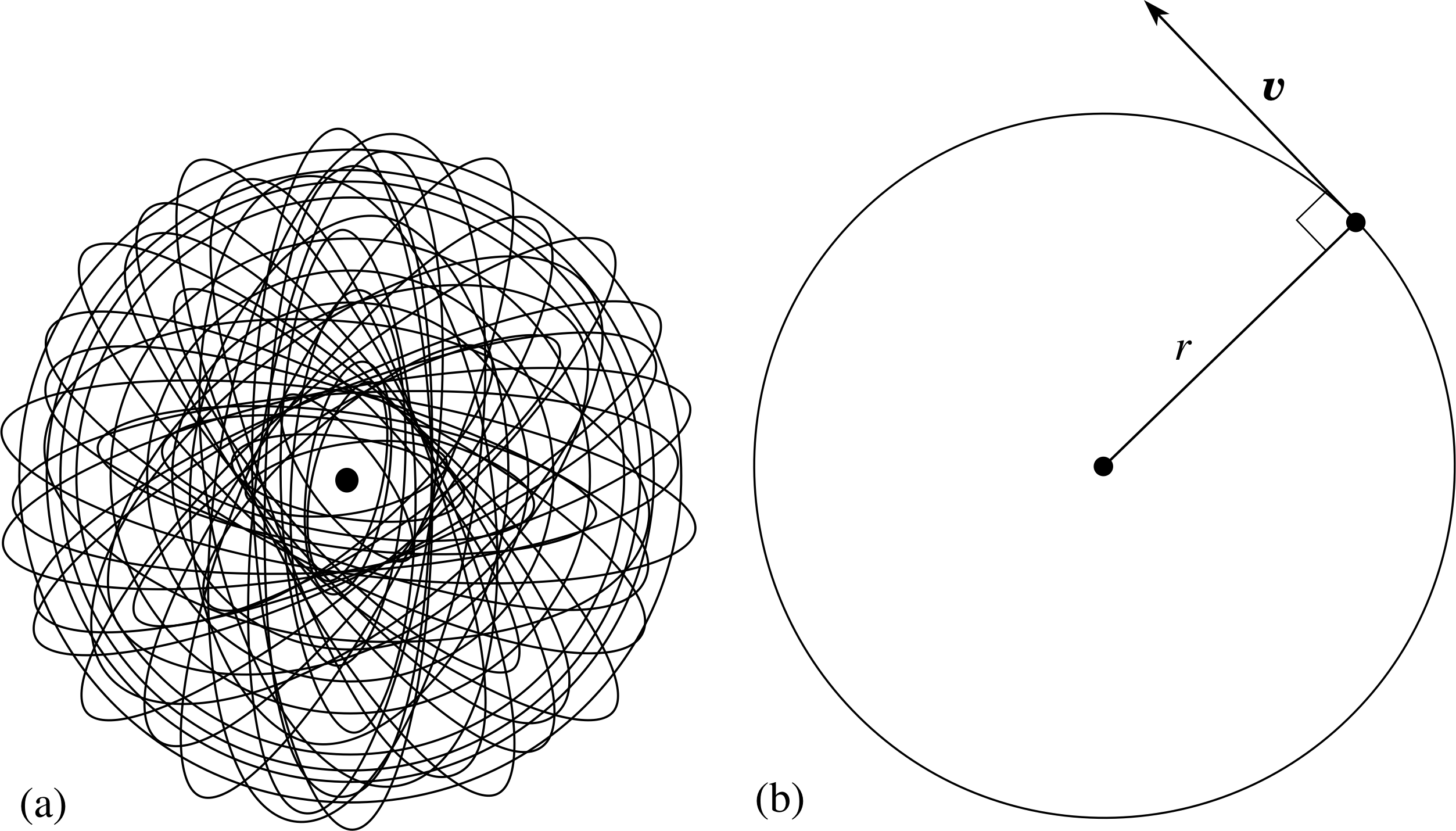
Figure 5 (a) Rutherford’s model of an atom, in which negatively charged electrons orbit a tiny, positively charged nucleus. (b) Bohr’s model of an atom, in which the electron moves with speed υ in a circular orbit of radius r around the nucleus.
In 1913, Niels Bohr opened up new vistas for atomic physics by formulating a new and extremely powerful model for the simplest atom of all – the hydrogen atom. Bohr’s model contained all the new ingredients required to derive many important features of the hydrogen atom, including Balmer’s formula. Bohr’s model also accurately predicted the wavelengths of all the other lines in the infrared and ultraviolet.
The model formulated by Bohr looks at first sight very similar to Rutherford’s model since in both of them the hydrogen atom consists of an electron orbiting a nucleus (Figure 5). Bohr’s innovation was to make some specific assumptions about the behaviour of the orbiting electron, and this made possible new insights into the properties of hydrogen. In this section, we define Bohr’s model of the hydrogen atom in terms of four postulates, that is, four statements that are assumed to be true for the purposes of developing the model.
Postulate 1 The electron in the atom moves in a circular orbit centred on the nucleus; the electric force between them is described by Coulomb’s law.
In this postulate, the nucleus is supposed to be so massive, compared with the electron, that it remains stationary while the electron is held in a circular orbit by the electrical attraction. This assumption is surely the simplest that could have been made. Let us now move on to consider the second postulate.
Postulate 2 The motion of the electron is described by Newton’s laws of motion in all but one respect – the magnitude L of the electron’s angular momentum is quantized in units of Planck’s constant h i divided by 2π, i.e.
$L = \dfrac{nh}{2\pi}$(2) i
where the number n, known as Bohr’s quantum number, can have any of the positive integer values, so n = 1 or 2 or 3, etc.
Equation 2 is known as Bohr’s quantization condition. In making this assumption, Bohr was asserting a remarkable new idea. He claimed that not only was the angular momentum of the orbiting electron about the nucleus constant but also that its magnitude was quantized, i.e. that it could take only certain definite values. When n = 1, L = h/2π, when n = 2, L = 2h/2π, and so on. This suggestion was extraordinary because it contradicted the assumption of Rutherford’s model (based on Newton’s laws of classical mechanics) that the electron should, in principle, have been able to have any value of angular momentum.
According to classical mechanics the magnitude of the electron’s angular momentum L, about the nucleus, is given by
L = merυ(3)
To see the implications of Bohr’s second postulate consider the quantities on the right–hand side of Equation 3. The mass me of the electron is fixed, although its speed υ and the radius r of its orbit are not. According to classical physics the speed and radius could vary continuously. Thus classical physics predicts that the electron’s angular momentum should, in principle, be able to take any value. Bohr’s assertion that L could not take any value, and that its possible values were restricted to those given by the quantization condition (Equation 2) implied corresponding restrictions on the orbital radius r and orbital speed υ of the electron.
Question T5
Confirm that the right–hand sides of Equations 2 and 3 can be measured in the same SI units.
Answer T5
The right–hand side of Equation 2,
$L = \dfrac{nh}{2\pi}$(Eqn 2)
has the same units as h since all the other quantities have no units. From the expression for the energy of a photon, E = hf, we see that h has SI units of J s. The right–hand side of Equation 3,
L = me rυ(Eqn 3)
has SI units of (kg)(m)(m s−1) = kg m2 s−1 = (kg m s−2)(m s) = N m s = J s. Notice that Planck’s constant has the same SI units as angular momentum.
Eqation 3) and the restricted values allowed for that quantity by the quantization condition (Equation 2) gives
$L = m_{\rm e}r\upsilon = \dfrac{nh}{2\pi}$
and therefore $r = \dfrac{nh}{2\pi m_{\rm e}\upsilon}$(4)
You will see shortly that the first two postulates imply that for each value of n there is only one possible value for the orbital radius r and for the orbital speed υ. Thus, to each value of n there corresponds a single well–defined orbit, called the nth Bohr orbit. You will also see that the greater the value of n that characterizes an orbit, the greater is that orbit’s radius. However, before proving these results, two more postulates are needed to define the model completely.
Postulate 3 Despite its acceleration, the electron does not continuously radiate electromagnetic energy, so its total energy (in each of its possible orbits) remains constant.
Classical physics forbids the stability of the Bohr atom, as it did for its predecessor, the Rutherford atom. Although the analogy between Bohr’s model of hydrogen and the planetary model of the Solar System is appealing, there is one fundamental distinction between them which is all important for the stability of the system. The problem is simply that, unlike the Earth in its orbit around the Sun, the electron is a charged particle. Classical Newtonian mechanics tells us that an orbiting particle accelerates towards the centre of the orbit and classical electromagnetism tells us that accelerating charges must emit electromagnetic radiation, which carries away energy.
In classical terms there is no escape from the conclusion that an orbiting electron will lose energy.i Since the hydrogen atom is stable this poses an insurmountable problem for classical physics.
Bohr’s postulate that the orbiting electron would not continuously emit electromagnetic radiation implied that the electron did not gradually lose its energy, which in turn implied that the total energy of the orbiting electron remained constant in each of the allowed orbits. i
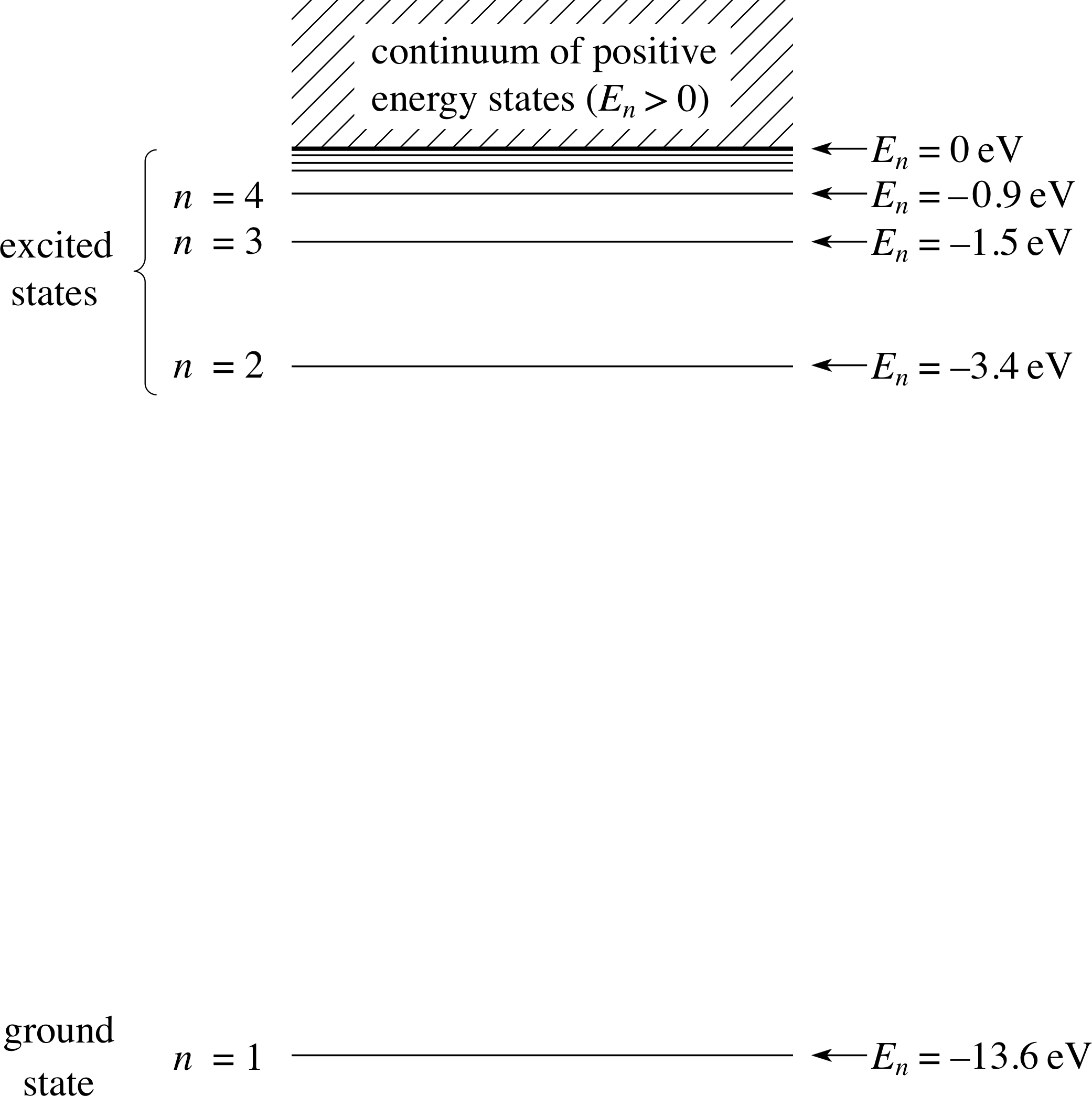
Figure 6 The energy level diagram for atomic hydrogen, extended to include the continuum.
This suggestion by Bohr introduced the idea that each orbit corresponded to a specific bound state for the electron in the atom, with each bound state having an associated energy level for the electron. The set of bound states, each with its particular energy level, can be depicted on an energy level diagram, such as that shown in Figure 6.
Figure 6 shows each bound state for atomic hydrogen, characterized by the integer value of n which determines the angular momentum of the electron via the quantization condition
$L = m_{\rm e}r\upsilon = \dfrac{nh}{2\pi}$
The energy levels for these bound states are written as En, with the bound state of lowest energy and lowest angular momentum (n = 1) referred to as the ground state and its energy as the ground level. Bound states of higher energies, corresponding to n = 2, 3, 4, 5, etc., are referred to as excited states and their energies as excited levels. When we return to Figure 6 next, you will be able to calculate the energy levels for all these bound states and to appreciate the other features of that figure, to which we have not yet referred.
The prediction that the energy of the electron was quantized was quite revolutionary. It used the developing ideas of quantum theory to provide a degree of stability for the atom that was not provided by purely classical models such as Rutherford’s. Although other cracks were appearing in classical physics at the time, the new quantum physics was not yet developed and Bohr sought to proceed by postulating that there was no radiation for those orbits in which the electron has the quantized values of angular momentum specified in Equation 2.
$L = \dfrac{nh}{2\pi}$(Eqn 2)
This postulate was a working hypothesis rather than a justifiable claim, to be judged according to whether predictions of the model agreed with experiment. Bohr’s model should only be considered as an interim one in which Bohr introduced quantization of angular momentum as the new quantum idea. Later, this basic idea was to prove to be a key feature in the development of the much more sophisticated quantum model of the atom. In today’s physics, the belief in the quantization of angular momentum for an electron in an atom lives on, long after the demise of Bohr’s model.
One question which has not yet been addressed is ‘What is the mechanism by which the hydrogen atom emits or absorbs its characteristic spectral lines?’ This question is answered by Bohr’s fourth and final postulate.
Postulate 4 When an electron that has energy Ei initially, in the orbit characterized by the Bohr quantum number ni, makes a transition to a new final orbit characterized by the Bohr quantum number nf, in which it has a lower energy Ef, a single quantum of electromagnetic radiation (a photon) is emitted. i This process is called an emission transition.
The frequency f of the associated radiation is given by the Planck–Einstein formula
$f = \dfrac{E_{\rm i}-E_{\rm f}}{h}$(5a)
This postulate identifies transitions between two bound states as corresponding to one definite emitted frequency or wavelength of light in the spectrum. It provides the vital link between the structure of the hydrogen atom and the quantum theory of electromagnetic radiation, as developed by Max Planck (1858–1947) and Albert Einstein (1879–1955). In this theory light interacts with atoms via the emission or absorption of photons, each of which carries a discrete amount of energy E = hf, where f is the frequency of the light and h is Planck’s constant. Bohr identified the photon energy as the difference between the two energy levels of the electron between which the transition occurs. According to Bohr, when an electron loses energy (Ei − Ef) by making a transition from the energy level Ei to the lower energy level Ef this energy is carried away by a single photon of electromagnetic radiation, the frequency of which is given by the Planck–Einstein formula.
Similarly, there are processes in which radiation is absorbed and the electron gains energy, making a transition from an initial energy level Ei to a higher final energy level Ef. This process is called an absorption transition.
For emission or absorption, the frequency of the radiation is given by
$f = \dfrac{\lvert\,E_{\rm i}-E_{\rm f}\,\rvert}{h}$(5b) i
and the wavelength λ of the radiation (λ = c/f) is given by
$\lambda = \dfrac{hc}{\lvert\,E_{\rm i}-E_{\rm f}\,\rvert}$(6)
where c is the speed of light in a vacuum.
Since the energies Ei and Ef of the electron can take only certain definite values (Postulate 3), it follows from Equations 5b and 6 that the wavelengths of electromagnetic radiation emitted or absorbed when the electron makes transitions between these energy levels also have only certain, definite values. This, according to Bohr’s theory, is why spectral lines are observed in emission or absorption. If energy is transferred to individual hydrogen atoms in a spectral lamp, many different emission transitions become possible and many different wavelengths of radiation (spectral lines) will be seen.
This concludes our discussion of the assumptions Bohr made in formulating his model of the hydrogen atom; they are summarized in Table 1.
| Formal statement of the postulate | Informal comments on the postulate and its implications | |
|---|---|---|
| Postulate 1 |
The electron in the atom moves in a circular orbit |
This postulate asserts that Coulomb’s (classical) law |
| Postulate 2 |
The motion of the electron is described by Newton’s |
Contrary to the expectations of classical physics, the |
| Postulate 3 |
Despite its acceleration, the electron does not |
Contrary to the expectations of classical physics, the |
| Postulate 4 |
When an electron that has total energy Ei, in the f = (Ei − Ef ) /h |
With this postulate, the idea of radiation quanta, or |
What is your reaction to the postulates? The most favourable view of them might be that they appear to constitute a plausible mixture of intuitively reasonable, classical ideas with the revolutionary quantum ideas of Planck and Einstein. On the other hand, you may think that the model is an artificial and illogical attempt to mix the unmixable – classical and quantum physics. Both of these attitudes are reasonable and justifiable, but it would be premature to pass final judgement on the model before its predictions have been compared with experiment. This will be done in the remainder of this section, but before you move on try Questions T6 and T7.
Question T6
State the four postulates that define Bohr’s model of the hydrogen atom. (Try to do this without looking them up! It doesn’t matter if you cannot quote the postulates word for word, but you should be able to recall their essential content.)
Answer T6
These are summarized in Table 1 at the end of Subsection 4.1.
Question T7
It was said that Bohr’s model might be regarded as an ‘attempt to mix the unmixable – classical and quantum physics’. For each of the four postulates that define the model, state whether it is based on purely classical physics, or on purely quantum physics, or on a mixture of the two.
Answer T7
In Table 1, Postulate 1 is a classical result; Postulate 2 is a mixture of classical physics (Newtonian mechanics) and quantum physics (quantized angular momentum); Postulate 3 is a quantum result and a denial of the classical result; Postulate 4 is a quantum result (interactions of an electromagnetic wave with an atom is via photons, emitted or absorbed), but having consistency with classical energy conservation.
4.2 Derivation of the allowed orbital radii
The discussions in Subsection 4.1, concerning the quantization of an electron’s orbital angular momentum, led us to the conclusion that
$L = m_{\rm e}r\upsilon = \dfrac{nh}{2\pi}$ i
and therefore $r = \dfrac{nh}{2\pi m_{\rm e}\upsilon}$(Eqn 4)
i.e.$\upsilon = \dfrac{nh}{2\pi m_{\rm e}r}$(7)
Equation 4 and Equation 7 both express the relationship between the radius r and the electron’s speed υ in any allowed orbit. We can arrive at another relationship between r and υ by considering the mechanics of circular motion under an electric force. In Bohr’s model of the atom the centripetal force, required to hold the electron in its circular orbit, is provided by the electrical attraction of the electron (charge −e) to the proton (charge +e).
Equating the magnitude of the centripetal force with that of the electric force from Coulomb’s law gives
$\dfrac{m_{\rm e}\upsilon^2}{r} = \dfrac{e^2}{4\pi\varepsilon_0r^2}$
where ε0 is the permittivity of free space.
Multiplying both sides of this equation by r gives
$m_{\rm e}\upsilon^2 = \dfrac{e^2}{4\pi\varepsilon_0r}$(8)
and substitution of υ from Equation 7 into Equation 8 gives
$m_{\rm e}\left(\dfrac{nh}{2\pi m_{\rm e}r}\right)^2 = \dfrac{e^2}{4\pi\varepsilon_0r}$
Multiplying both sides of this equation by 4πr leads to
$\dfrac{n^2h^2}{\pi m_{\rm e}r} = \dfrac{e^2}{\varepsilon_0}$
so$r = n^2\left(\dfrac{\varepsilon_0h^2}{\pi m_{\rm e}e^2}\right) = n^2a_0$(9) i
where the constant quantity $\left(\dfrac{\varepsilon_0h^2}{\pi m_{\rm e}e^2}\right)$ has been written as a0.
Let us pause here for a while and explore this result. Try the next two questions before you proceed further.
Question T8
Determine the units of the quantity in the brackets in Equation 9.
Does this agree with the units you would expect for a0 on the basis that Equation 9 also claims that r = n2a0?
(Use the data given in the margin note.) i
Answer T8
Equation 9 is
$r = n^2\left(\dfrac{\varepsilon_0h^2}{\pi m_{\rm e}e^2}\right) = n^2a_0$(Eqn 9)
The list of fundamental physical constants gives the SI units for ε0, h, me and e. The quantity in brackets is then seen to have SI units:
$\rm \dfrac{(C^2\,N^{-1}\,m^{-2})\,N^2\,m^2\,s^2}{kg\,C^2} = \dfrac{N\,s^2}{kg} = \dfrac{(kg\,m\,s^{-2})s^2}{kg} = m$
This is as expected since the quantity in brackets is also a0, the radius of the ground state orbit in the hydrogen atom.
Question T9
Determine the magnitude (in SI units) of a0. What is the physical significance of this quantity?
Answer T9
The magnitude of the quantity in brackets in Equation 9,
$r = n^2\left(\dfrac{\varepsilon_0h^2}{\pi m_{\rm e}e^2}\right) = n^2a_0$(Eqn 9)
is:
$\dfrac{\varepsilon_0h^2}{\pi m_{\rm e}e^2} = \rm \dfrac{8.85\times10^{-12}\times(6.63\times10^{-34})^2}{3.14\times9.11\times10^{-31}\times(1.60\times10^{-19})^2}\,m = 5.3\times10^{-11}\,m$
The physical significance of this is that it is Bohr’s prediction for the radius of the electron’s orbit in the hydrogen atom in its ground state (where n = 1).
| Bohr orbit | Radius of orbit/10−10 m |
|---|---|
| n = 1 | a0 = 0.53 |
| n = 2 | r = 2.1 |
| n = 3 | r = 4.8 |
| n = 4 | r = 8.5 |
The radius of the n = 1 orbit is usually called the Bohr radius and is denoted by a0. As pointed out in Answer T9 it represents the radius of the n = 1 orbit in Bohr’s model of the hydrogen atom. Table 2 shows the radii of the first four Bohr orbits for the electron in atomic hydrogen.
Notice how quickly the radii increase with n.
4.3 Derivation of the electron’s orbital speed
In Subsection 4.2 we arrived at an expression for the allowed radii of the Bohr orbits. We already know that in a Bohr orbit the electron’s speed υ and the orbital radius r are connected through
i.e.$\upsilon = \dfrac{nh}{2\pi m_{\rm e}r}$(Eqn 7)
Substituting for r, using
$r = n^2\left(\dfrac{\varepsilon_0h^2}{\pi m_{\rm e}e^2}\right) = n^2a_0$(Eqn 9) i
produces
$\upsilon = \left(\dfrac{nh}{2\pi m_{\rm e}}\right)\left(\dfrac{\pi m_{\rm e} e^2}{n^2\varepsilon_0h^2}\right) = \dfrac{e^2}{2\varepsilon_0h}\left(\dfrac1n\right)$(10)
✦ In which Bohr orbit does the electron have the largest kinetic energy?
✧ The kinetic energy is mυ2/2 and from Equation 10,
$\upsilon = \left(\dfrac{nh}{2\pi m_{\rm e}}\right)\left(\dfrac{\pi m_{\rm e} e^2}{n^2\varepsilon_0h^2}\right) = \dfrac{e^2}{2\varepsilon_0h}\left(\dfrac1n\right)$(Eqn 10)
the speed υ is largest when n is as small as possible, i.e. when n = 1; this is in the first Bohr orbit. This may surprise you, as may the related idea that as you move the electron to larger and larger orbits the kinetic energy tends to zero. However, it is not so surprising when you realize that, in this limit, the electron must be unaware of the nucleus, since the electric force has shrunk to zero; the electron is now free from the atom and can be at rest, with zero kinetic energy.
4.4 Derivation of the kinetic, potential and total energies of an electron
Our purpose in this subsection is to determine the total energy of the electron in each of the bound states of the hydrogen atom, according to Bohr’s model. Since the total energy involves the sum of the kinetic energy and the electric potential energy, we must now calculate both of these for each Bohr orbit. The kinetic energy depends on the speed of the electron in the orbit and we have an expression for υ in Equation 10,
$\upsilon = \left(\dfrac{nh}{2\pi m_{\rm e}}\right)\left(\dfrac{\pi m_{\rm e} e^2}{n^2\varepsilon_0h^2}\right) = \dfrac{e^2}{2\varepsilon_0h}\left(\dfrac1n\right)$(Eqn 10)
The electric potential energy depends on the distance r of the electron from the nucleus and we have an expression for this distance in Equation 9,
$r = n^2\left(\dfrac{\varepsilon_0h^2}{\pi m_{\rm e}e^2}\right) = n^2a_0$(Eqn 9)
The kinetic energy Ekin is given by the expression
$E_{\rm kin} = \dfrac12m_{\rm e}\upsilon^2 = \dfrac12 m_{\rm e}\left(\dfrac{e^2}{2\varepsilon_0hn}\right)^2 = \dfrac{m_{\rm e} e^4}{8\varepsilon_0^2h^2}\left(\dfrac{1}{n^2}\right)$(11)
The potential energy Epot is given by the expression
$E_{\rm pot} = -\dfrac{e^2}{4\pi\varepsilon_0r} = -\dfrac{e^2}{4\pi\varepsilon_0}\left(\dfrac{\pi m_{\rm e}e^2}{\varepsilon_0h^2n^2}\right) = -\dfrac{m_{\rm e}e^4}{4\varepsilon_0^2h^2}\left(\dfrac{1}{n^2}\right)$(12)
The total energy in the nth Bohr orbit En is the sum of Equations 11 and 12 and is given by
$E_n = E_{\rm kin} + E_{\rm pot} = \dfrac{m_{\rm e}e^4}{4\varepsilon_0^2h^2}\left(\dfrac{1}{n^2}\right)(1-2)$
$E_n = - \dfrac{m_{\rm e}e^4}{4\varepsilon_0^2h^2}\left(\dfrac{1}{n^2}\right)$(13)
Before we look at the details of these results it is important to appreciate some general features.
- 1
-
Both kinetic and potential energy depend on n in the same way – they are proportional to 1/n2.
- 2
-
Although kinetic energy (which depends on υ2) can only be positive, the potential energy (which involves the attraction of opposite charges) is negative. This is a consequence of the zero of potential energy being taken to be where the two charges are infinitely separated; the potential energy then becomes more negative as the two attracting charges approach each other.
- 3
-
For any bound state (Bohr orbit) the magnitude of the potential energy is twice that of the kinetic energy. i
- 4
-
Because Epot = −Ekin the total energy in a bound state is always negative, with the ground state (innermost orbit) having the largest negative energy. The zero of total energy corresponds to n = ∞, with the electron at rest (Ekin = 0) at an infinite distance from the nucleus (Epot = 0).
✦ What would you expect to be the units of the coefficient $\dfrac{m_{\rm e}e^4}{4\varepsilon_0^2h^2}$ in Equation 13?
✧ Since En is an energy and n has no units, it follows that the coefficient itself must be an energy, and in SI units it will be measured in joules.
Question T10
Determine the magnitude (in SI units) of $\dfrac{m_{\rm e}e^4}{4\varepsilon_0^2h^2}$.
Calculate its value in electronvolts (eV).
What is the physical significance of this quantity?
Answer T10
The magnitude of the quantity is
$\dfrac{m_{\rm e}e^4}{8\varepsilon_0^2h^2} = \rm \dfrac{9.11\times10^{-31}\times(1.60\times10^{-19})^4}{8(8.85\times10^{-12})^2(6.63\times10^{-34})^2}\,J = 2.17\times10^{-18}\,J = 13.6\,eV$
The quantity 13.6 eV represents the energy below zero of the ground state. (This calculation may cause problems for your calculator, depending on the order in which you carry out the calculation.)
4.5 The energy level diagram for atomic hydrogen; unbound states and ionization
If we combine the result of Question T10 with Equation 13,
$E_n = - \dfrac{m_{\rm e}e^4}{4\varepsilon_0^2h^2}\left(\dfrac{1}{n^2}\right)$(Eqn 13)
we arrive at a very important expression for the energy levels for the bound states of atomic hydrogen, expressed either in terms of fundamental constants or in electronvolts (in a form that is easier to recall). This is given in Equation 14,
$E_n = -\dfrac{m_{\rm e}e^4}{4\varepsilon_0^2h^2}\left(\dfrac{1}{n^2}\right) = -\left(\dfrac{13.6}{n^2}\right)\,{\rm eV}$(Eqn 14) i
The Bohr orbits represent bound states of the electron in the hydrogen atom. Bound states always have a total energy which is negative. This signals that energy must be added to the electron to remove it from the atom. When the electron is removed, a positively charged hydrogen ion is left and the atom is said to have been ionized. The minimum energy required to just remove a ground state electron is called the ionization energy or the ionization potential of the atom. This minimum energy will leave the electron at rest at infinity – with zero kinetic energy, zero potential energy and total energy En = 0. Equation 14 can describe this electron energy if we take the limiting case as n approaches ∞ (n → ∞).
The energy level corresponding to the limit where En → 0 as n → ∞ is called the ionization level. Equation 14 identifies the ionization potential of atomic hydrogen as 13.6 eV.
Figure 6 The energy level diagram for atomic hydrogen, extended to include the continuum.
If the electron is given more energy than is required to reach the ionization level then it will escape from the atom and have net kinetic energy, but its potential energy remains at zero since it is still outside the influence of the nucleus. In this situation the electron moves freely with speed υ and it is now said to be in an unbound state. In such a state its kinetic energy mυ2/2 may have any positive value.
Thus discrete or quantized energy levels are characteristic of bound states whereas unbound ‘states’ can have any positive energy; unbound states are said to be states lying in the continuum, which is a continuous range of states of all possible positive energies which lie above the ionization level at En = 0.
This situation is depicted on the extended energy level diagram shown in Figure 6.
Equation 14, together with its illustration in Figure 6, is extremely important since it gives the Bohr model’s prediction for the bound state energy levels of the electron in a hydrogen atom.
Look carefully at Figure 6 – it has a number of important features which we can appreciate qualitatively, even before we make detailed calculations:
- 1
-
From Equations 5b and 6
$f = \dfrac{\lvert\,E_{\rm i}-E_{\rm f}\,\rvert}{h}$(Eqn 5b)
$\lambda = \dfrac{hc}{\lvert\,E_{\rm i}-E_{\rm f}\,\rvert}$(Eqn 6)
we know that transitions between pairs of bound states will give rise to spectral lines; the larger the energy difference between these bound states the higher will be the frequency of light emitted or absorbed. It is the energy gaps between pairs of energy levels in Figure 6 that are important, though transitions are not, of course, confined to being between adjacent levels. We will examine these transitions in detail in the next subsection.
- 2
-
As n → ∞ the energy levels become closer and closer together, with the energy difference between adjacent levels shrinking to zero as the levels converge to the ionization level at En = 0.
- 3
-
Equation 9,
$r = n^2\left(\dfrac{\varepsilon_0h^2}{\pi m_{\rm e}e^2}\right) = n^2a_0$(Eqn 9)
shows that as n→∞ the orbits themselves become further and further apart, with both the radii of the Bohr orbits and the differences between the radii of adjacent orbits increasing without limit.
- 4
-
Because the energies are proportional to 1/n2, the convergence of the energy levels is quite rapid. If we sit at any particular level, then the energy gap between this level and the next highest level forms a substantial fraction of the energy gap to the ionization level – you can see this quite strikingly if you look at the gap between n = 1 and n = 2 and compare it with the gap between the n = 1 level and the ionization level.
- 5
-
Above the ionization level the hatching in the diagram indicates a continuous range of available energies (the continuum); in this region, the positive energy corresponds to an unbound electron which is free to leave the atom, carrying with it some excess kinetic energy.
- 6
-
It is interesting to note that bound states can exist, in principle, for very large values of n and that atoms of hydrogen in such states could have quite large radii; such atoms are referred to as Rydberg atoms, named after the Swedish physicist Johannes Rydberg (1854–1919). Rydberg atoms have been detected in space, on the basis of their spectra. It is possible, in principle, to imagine a hydrogen atom with an orbit radius of several metres! The story of Rydberg atoms is a fascinating one but unfortunately we have no time here to take it further.
Question T11
(a) Is it correct to say that the total energy of an unbound electron is quantized? Explain your answer.
(b) What would happen if 4 eV of energy were transferred to an electron in the n = 2 energy level of a hydrogen atom?
Answer T11
(a) No, the statement is incorrect since an unbound electron has a total energy which is positive and it thus lies above the ionization limit, in the continuum of states with positive energy. An unbound electron is a free electron; its potential energy, well away from the nucleus, is zero and its kinetic energy can have any positive value. It is only bound electrons which have definite or discrete energy levels.
(b) The electron in the bound state with n = 2 has a negative energy given by Equation 13,
$E_n = - \dfrac{m_{\rm e}e^4}{4\varepsilon_0^2h^2}\left(\dfrac{1}{n^2}\right)$(Eqn 13)
with n = 2 substituted
∴$E_2 = -\left(\dfrac{13.6}{2^2}\right)\,{\rm eV} = -3.40\,{eV}$
When 4 eV is added to this energy the electron reaches a total energy of +0.60 eV which puts the electron into the continuum, free from the atom, with a kinetic energy of 0.60 eV. The speed of the free electron could be calculated using Ekin = mυ2/2.
4.6 Transitions, spectral lines and Balmer’s formula
Bohr’s model implies that each line seen in the hydrogen spectrum should be identified with a transition from one energy level to another. Emission lines are the result of transitions in which the electron loses energy by moving from states of relatively high energy to states of lower energy. Absorption lines are the result of transitions in which the electron gains energy by moving from states of relatively low energy to states of higher energy.
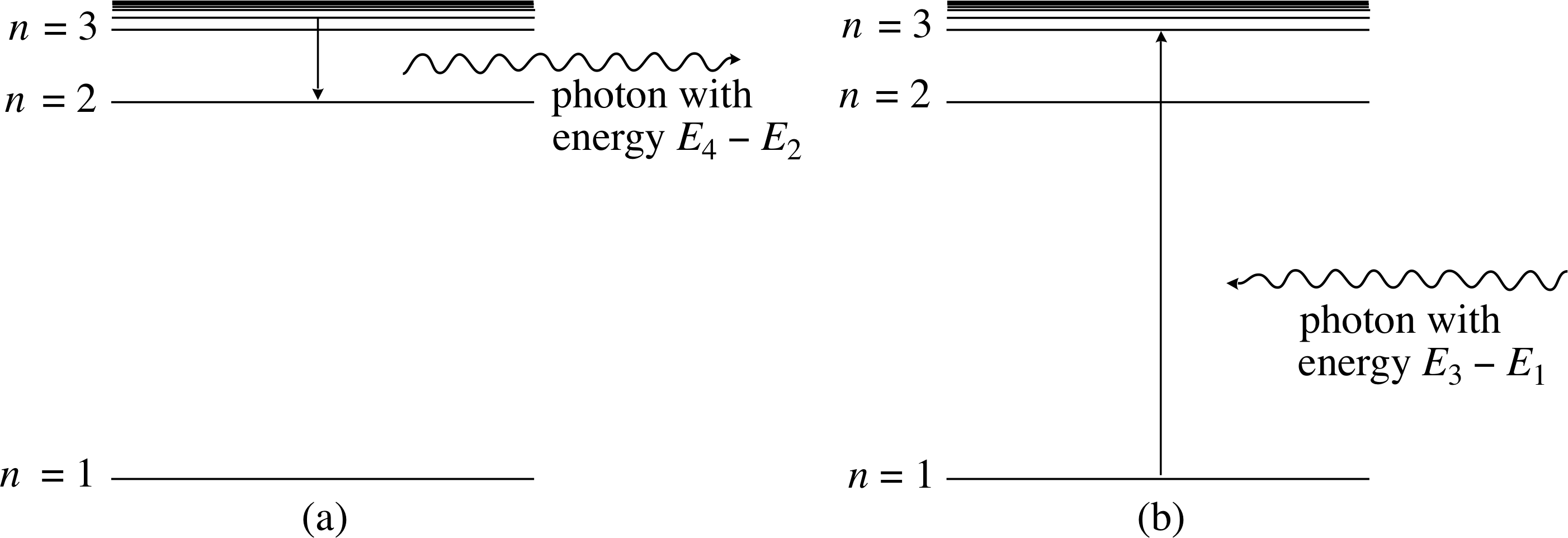
Figure 7 Emission and absorption transitions in atomic hydrogen, shown on the energy level diagram. (a) An emission process is one in which the electron makes a transition to a lower energy level, with the energy difference carried away by an emitted photon. (b) An absorption process is one in which the electron absorbs sufficient energy from an incident photon to move to a higher energy level.
Both emission and absorption transitions can be shown on the energy level diagram by vertical arrows connecting the two energy levels, as in Figure 7, with an arrowhead indicating the direction of the energy change for the electron.
The strong convergence of the energies with 1/n2 suggests a convenient way of grouping the possible transitions into several separate series of lines, where all members of a given series have the same lower level for their transitions. The region of the electromagnetic spectrum in which a particular series lies is set primarily by the energy of the lowest energy transition in the series. Figure 8 shows an example of such a series, in this case consisting of all transitions terminating on the n = 2 level. This series is in fact the Balmer series. Similar sets of transitions down to the n = 1 level produce the Lyman series in the far UV. Transitions down to the n = 3 level produce the Paschen series in the IR and there are many other series in the IR which are characterized by transitions down to lower levels which have n > 3. (The Lyman and Paschen series were introduced in Subsection 3.2.)
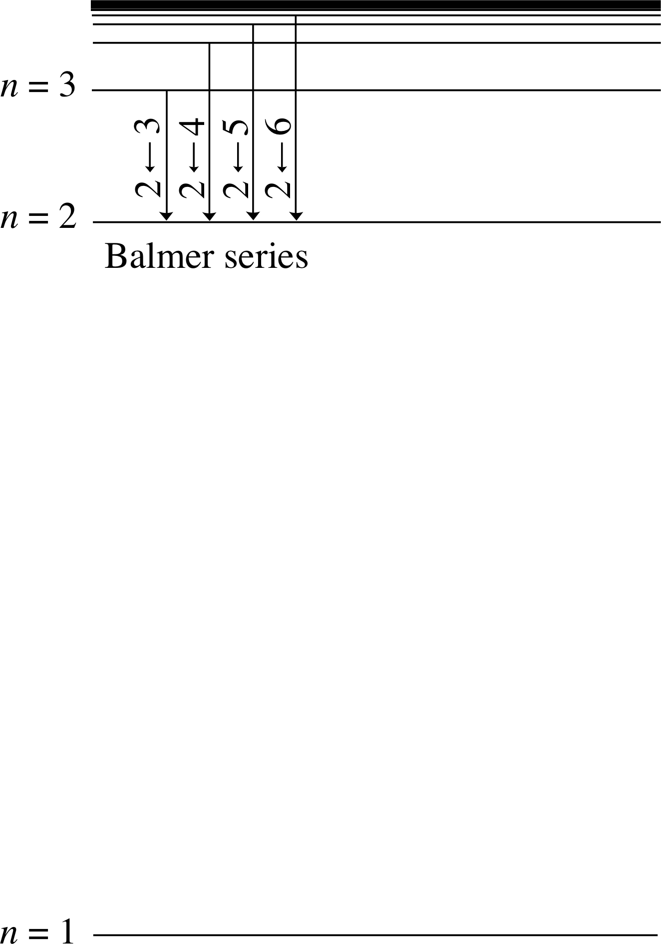
Figure 8 The set of all emission transitions down to the n = 2 level produces the Balmer series of lines in the visible part of the spectrum.
We can predict the wavelengths of the spectral lines of atomic hydrogen by using Equations 14, 5b and 6. For convenience we have collected them together.
$E_n = -\dfrac{m_{\rm e}e^4}{4\varepsilon_0^2h^2}\left(\dfrac{1}{n^2}\right) = -\left(\dfrac{13.6}{n^2}\right)\,{\rm eV}$(Eqn 14)
For emission or absorption, the frequency and wavelength of the radiation are given by
$f = \dfrac{\lvert\,E_{\rm i}-E_{\rm f}\,\rvert}{h}\quad\text{and}\quad\lambda = \dfrac{hc}{\lvert\,E_{\rm i}-E_{\rm f}\,\rvert}$(Eqns 5b and 6)
where c is the speed of light in a vacuum, Ei is the energy of the initial level with n = ni and Ef is that of the final level with n = nf. From Equation 14 we can see that
$\lvert\,E_{\rm i}-E_{\rm f}\,\rvert = 13.6\,\left\lvert\,\dfrac{1}{n_{\rm f}^2} - \dfrac{1}{n_{\rm i}^2}\,\right\rvert\,{\rm eV} = \left(\dfrac{m_{\rm e}e^4}{8\varepsilon_0^2h^2}\right)\,\left\lvert\,\dfrac{1}{n_{\rm f}^2} - \dfrac{1}{n_{\rm i}^2}\,\right\rvert$(15)
We can now write down the frequency, fi → f, and wavelength, λi → f, for the i → f transition.
In order that frequencies and wavelengths are correct in SI units, the energies must be expressed in joules not electronvolts.
Thus$f_{\rm i\to f} = \dfrac{\lvert\,E_{\rm i}-E_{\rm f}\,\rvert}{h} = \left(\dfrac{m_{\rm e}e^4}{8\varepsilon_0^2h^2}\right)\,\left\lvert\,\dfrac{1}{n_{\rm f}^2} - \dfrac{1}{n_{\rm i}^2}\,\right\rvert$(16)
and$\lambda_{\rm i\to f} = \dfrac{c}{f_{\rm i\to f}} = \left(\dfrac{8\varepsilon_0^2h^2}{m_{\rm e}e^4}\right)\,\left\lvert\,\left(\dfrac{1}{n_{\rm f}^2} - \dfrac{1}{n_{\rm i}^2}\right)^{-1}\,\right\rvert = \left(\dfrac{8\varepsilon_0^2h^2}{m_{\rm e}e^4}\right) \left(\dfrac{n_{\rm i}^2n_{\rm f}^2}{\lvert\,n_{\rm i}^2-n_{\rm f}^2\,\rvert}\right)$(17)
Spectroscopic measurements of wavelengths are among the most precise measurements in science. Equation 17 relates measured wavelengths to the fundamental constants of nature, me, e, ε0, h and c, using known integers, ni and nf, in which there are no experimental uncertainties. The attraction then is to use spectroscopy to measure precisely the particular combination of fundamental constants which appears in Equation 17. This result can then be combined with the results of other precise experiments depending on these same fundamental constants to obtain precise values for the fundamental constants themselves. This is exactly what has been done to determine our present ‘best values’ for the fundamental constants.
Spectroscopy has played a vital part in this process and a convenient stepping stone in this is the measurement of Rydberg’s constant, which is a convenient combination of the fundamental constants, defined as:
$R = \dfrac{m_{\rm e}e^4}{8\varepsilon_0^2h^3c}$(18)
The current value for Rydberg’s constant is R = 1.097 37 × 107 m−1. The number of significant figures here underlines the precision of spectroscopy. i
It is now time to test Bohr’s model in terms of the known Balmer lines and to see whether we can derive the ‘mysterious’ formula of Balmer. This is so important that it is appropriate that you do it yourself. Here’s your chance!
Question T12
Use Bohr’s model, with the value of the Rydberg’s constant just given, to calculate the wavelengths of the first four members of the Balmer series. Compare these with the experimental values from Subsection 3.1 [wavelengths 656.21 nm (red), 486.07 nm (blue/green), 434.01 nm (blue/violet) and 410.12 nm (violet)] and those calculated in Question T3 [wavelengths 656.21 nm (red), 486.08 nm (blue/green), 434.00 nm (blue/violet) and 410.13 nm (violet).]
Answer T12
We can use Equation 17,
$\lambda_{i\to f} = \dfrac{c}{f_{\rm i\to f}} = \left(\dfrac{8\varepsilon_0^2h^2}{m_{\rm e}e^4}\right)\,\left\lvert\,\left(\dfrac{1}{n_{\rm f}^2} - \dfrac{1}{n_{\rm i}^2}\right)^{-1}\,\right\rvert = \left(\dfrac{8\varepsilon_0^2h^2}{m_{\rm e}e^4}\right) \left(\dfrac{n_{\rm i}^2n_{\rm f}^2}{\lvert\,n_{\rm i}^2-n_{\rm f}^2\,\rvert}\right)$(Eqn 17)
with the value of Rydberg’s constant given at the end of Subsection 4.6, to calculate the wavelengths of the first four lines (nf = 2 and ni = 3, 4, 5 and 6)
$\lambda_{\rm i\to f} = \dfrac{1}{1.09737\times10^7}\left(\dfrac{n_{\rm i}^2n_{\rm f}^2}{n_{\rm i}^2-n_{\rm f}^2}\right)\,{\rm m} = 9.112\,70\times10^{-8}\left(\dfrac{n_{\rm i}^2n_{\rm f}^2}{n_{\rm i}^2-n_{\rm f}^2}\right)\,{\rm m}$
For ni = 3, $\lambda_{3\to 2} = \rm 91.127\,0\left(\dfrac{9\times4}{9-4}\right)\,nm = 656.114\,nm$
For ni = 4, $\lambda_{4\to 2} = \rm 91.127\,0\times\left(\dfrac{16\times4}{16-4}\right)\,nm = 486.011\,nm$
For ni = 5, $\lambda_{5\to 2} = \rm 91.127\,0\times\left(\dfrac{25\times4}{25-4}\right)\,nm = 433.938\,nm$
For ni = 6, $\lambda_{6\to 2} = \rm 91.127\,0\times\left(\dfrac{36\times4}{36-4}\right)\,nm = 410.72\,nm$
These Bohr predictions are in excellent agreement with the measured wavelengths given in Subsection 3.1 as 656.21 nm (red), 486.07 nm (blue/green), 434.01 nm (blue/violet) and 410.12 nm (violet). They are not quite in such good agreement with the experimental values as were Balmer’s formula results (656.21 nm, 486.08 nm, 434.00 nm and 410.13 nm), but the latter formula had no theoretical justification.
Comment You may notice that these Bohr values here are systematically low. They can be brought into even closer agreement with experiment by applying the small correction due to the finite mass of the nucleus (referred to in the marginal comment at the end of Subsection 4.6).
Question T13
Use the Bohr model results to derive Balmer’s formula.
Answer T13
Using the result derived in Answer T12
$\lambda_{\rm i\to f} = 91.127\,0\left(\dfrac{n_{\rm i}^2n_{\rm f}^2}{n_{\rm i}^2-n_{\rm f}^2}\right)\,{\rm nm}$
For nf = 2 and ni = n
$\lambda_{n\to2} = 91.127\,0\left(\dfrac{4n^2}{n^2-4}\right)\,{\rm nm} = 364.508\,\left(\dfrac{n^2}{n^2-4}\right)\,{\rm nm}$
This is Balmer’s formula, except for a small difference in the numerical factor.
An interpretation of the mysterious number n in Balmer’s formula can now be given – according to Bohr’s model, it denotes the Bohr quantum number, ni, of the upper energy level from which the electron makes its transition to the lower energy level, characterized by the Bohr quantum number nf = 2. You may already have anticipated some of this in Subsection 3.2, in your answer to Question T4.
Figure 8 The set of all emission transitions down to the n = 2 level produces the Balmer series of lines in the visible part of the spectrum.
4.7 Bohr’s model for the other series in the hydrogen spectrum
Without further discussion we can now explain all the other lines in the hydrogen spectrum (IR and UV) by appropriate choices of ni and nf in Bohr’s model. We note that the Balmer series appears in the visible because of the size of the dominant energy level spacing involved (n = 3 to n = 2). Similarly, the first member of the Lyman series (n = 2 to n = 1) puts this series into the far UV and the first member of the Paschen series (n = 4 to n = 3) puts this series into the IR. In Subsection 3.2 we gave the wavelengths of the first member of each of the Lyman and Paschen series. It is important now to test whether Bohr’s model is able to predict the wavelengths of these lines and of some other members of these series.
Question T14
In 1908, five years before Bohr developed his model, the German physicist Friedrich Paschen (1865–1947) observed two IR lines with wavelengths of 1 875.1 nm and 1 281.8 nm. Use Bohr’s model to show that these lines are the first two members of the series due to transitions down to the level with n = 3. Mark these transitions on Figure 8.
Answer T14
We can use the Bohr model to predict the wavelengths of any line in the hydrogen spectrum, given the values of niand nf. In particular, for the Paschen series we note that nf = 3. The predicted wavelengths are:
$\lambda_{\rm i\to f} = 91.127\,0\left(\dfrac{n_{\rm i}^2n_{\rm f}^2}{n_{\rm i}^2-n_{\rm f}^2}\right)\,{\rm nm}$
For nf = 3 and ni = n
$\lambda_{n\to2} = 91.127\,0\left(\dfrac{9n^2}{n^2-9}\right)\,{\rm nm} = 820.143\left(\dfrac{n^2}{n^2-9}\right)\,{\rm nm}$
For n = 4, $\lambda_{4\to3} = \rm 820.143\left(\dfrac{16}{16-9}\right)\,nm = 1\,874.6\,nm$
For n = 5, $\lambda_{5\to3} = \rm 820.143\left(\dfrac{25}{25-9}\right)\,nm = 1\,281.47\,nm$
The closeness of these predictions to the measured line wavelengths confirms their origin. Your diagram should now show the two added transitions as vertical lines connecting n = 4 to n = 3 and n = 5 to n = 3.
Now that you have done Question T14, Figure 8 should show two series of lines that were accounted for by Bohr’s model. With these successes behind him, Bohr confidently predicted the wavelengths of other series that he suggested should be detectable. For example, he predicted that there should be a series of lines corresponding to transitions to the ground state, n = 1. It was the physicist Theodore Lyman (1874–1954) who detected the first two lines in this series.
Question T15
Use Bohr’s model to find the first three lines in the far UV series (Lyman series). Mark these transitions on Figure 8.
Answer T15
The Lyman series in emission are transitions down to nf = 1. As in Question T14, the wavelengths for the lines in the Lyman series are given by
$\lambda_{\rm i\to f} = 91.127\,0\left(\dfrac{n_{\rm i}^2n_{\rm f}^2}{n_{\rm i}^2-n_{\rm f}^2}\right)\,{\rm nm}$
For nf = 1 and ni = n
$\lambda_{n\to1} = 91.127\,0\,\left(\dfrac{n^2}{n^2-1}\right)\,{\rm nm}$
For n = 2, $\lambda_{2\to1} = \rm 91.127\,0\left(\dfrac{4}{4-1}\right)\,nm = 121.503\,nm$
For n = 3, $\lambda_{3\to1} = \rm 91.127\,0\left(\dfrac{9}{9-1}\right)\,nm = 102.518\,nm$
For n = 4, $\lambda_{4\to1} = \rm 91.127\,0\left(\dfrac{16}{16-1}\right)\,nm = 97.202\,1\,nm$
These transitions should be marked on Figure 8, as n = 2 to n = 1 and n = 3 to n = 1 and n = 4 to n = 1.
Your Figure 8 now should show a fairly comprehensive amount of information about the spectrum of atomic hydrogen.
5 Production of spectra; excitation by heating and by collisions i
Figure 6 The energy level diagram for atomic hydrogen, extended to include the continuum.
At the end of Subsection 2.3 it was pointed out that a striking difference between the emission and absorption spectra of an element was that the emission spectrum contains many more lines, including all the lines which are seen in absorption. The energy scale of Figure 6 allows us to understand this observation, at least in relation to atomic hydrogen.
Hydrogen atoms will be in their ground states unless energy is transferred to them from some external source. The process of transferring energy to the atom is called excitation and will result in the atom making a transition from the ground state to one of the available excited states, from which it can then emit radiation in a transition to a lower level. Absorption of radiation is one such excitation process, but this is only effective if the photon energy is matched to the energy difference between the two energy levels concerned. Heating is another method of excitation; when a gas is heated the random molecular motion becomes more energetic and energy can be transferred to excitation of the atoms via collisions between them. Another excitation process involves collisions of the atoms with electrons in a beam.
Figure 6 shows that for a hydrogen atom to be excited out of its ground state, it must receive additional energy to reach at least the first excited state. This minimum energy is (E2 − E1) and in collisions this energy must come from the kinetic energies of the colliding partners. If the total kinetic energy available is less than (E2 − E1) then excitation cannot occur and the atoms remain in their ground state after the collision. To assess the chances of excitation in collisions we need to estimate the kinetic energies of the colliding partners and compare their sum with (E2 − E1).
Atoms or molecules in a gas are in random motion, with a range of speeds and kinetic energies. The average kinetic energy per particle is determined by the temperature of the gas, and is of the order of kT, where k is a fundamental physical constant known as Boltzmann’s constant i and T is the absolute temperature. Unless kT is comparable with (E2 − E1), excitation via collisions between atoms is very unlikely. So only when the temperature T of the gas is comparable with (E2 − E1)/k will significant excitation via collisions between the particles occur. Let us investigate the temperatures required for this.
Question T16
Calculate the minimum energy (E2 − E1) (in electronvolts and in SI units) needed to excite a hydrogen atom from its ground state to its first excited state. If Boltzmann’s constant k = 1.38 × 10⁻²³ J K−1, calculate the ratio (E2 − E1)/kT when the gas is at 2 000°C.
Answer T16
Using the result for E2 = −3.40 eV from Figure 6 and with E1 = −13.6 eV, the energy difference required is
E2 − E1 = (13.6 − 3.40) eV = 10.2 eV = 1.63 × 10⁻⁸ J
At 2 000 °C, i.e. T = 2 273 K,
kT = (1.38 × 10−23 × 2 273) J = 3.14 × 10⁻²⁰ J
∴$\dfrac{E_2-E_1}{kT} = \rm \dfrac{1.63\times10^{-18}\,J}{3.14\times10^{-20}\,J} = 51.9$
To be a little more quantitative we can draw on a result from statistical mechanics, i which tells us the ratio of the numbers of particles, N2/N1, having energies E2 and E1 when the temperature of the gas is T (T is measured in kelvin) is given by
$\dfrac{N_2}{N_1} = \exp\left[\dfrac{-(E_2-E_1)}{kT}\right]$(19)
Question T17
Use Equation 19 to calculate the relative numbers of hydrogen atoms in the first excited state and the ground state, when the gas is at 2 000°C. Comment on this result.
Answer T17
We use the result from Answer T16 at 2 000°C to obtain
$\dfrac{N_2}{N_1} = \exp(-51.9) = 2.88\times10^{-23}$
This is an extremely small probability.
It could be put in a striking way by observing that if ten litres of hydrogen gas, containing about 3 × 10²³ molecules or 6 × 10²³ atoms, were held at 2 000°C then there would be on average only about 1 or 2 excited atoms!
This probability is a very sensitive function of temperature, as you can see from the exponential dependence of the expression.
Although our calculations here have concerned hydrogen, the scale of the energy level diagrams for other atoms is similar, and typical excitation energies required are of the order of a few electronvolts. It is thus generally true that excitation of atoms by simple heating of the gas requires extremely high temperatures. Fortunately there is a much simpler method available.
Unlike neutral atoms, charged electrons can be accelerated up to large kinetic energies rather easily. A beam of electrons emitted from a heated filament can be accelerated through a potential difference of a few volts to produce electron kinetic energies which are able to excite atoms via collisions. This method does not require the atomic vapour to be heated to high temperatures and is the preferred method used in most spectral lamps. This justifies the assertions concerning spectral lamps, made at the end of Subsection 2.1.
We can now understand also why the absorption spectrum normally contains far fewer lines than the emission spectrum of the same element (as stated in Subsection 2.3). The explanation is simply that at all reasonable temperatures, almost all the atoms are in the ground state and absorption transitions therefore generally must start from the ground state. In contrast, in a spectral lamp, the excitation of atoms via electron collisions populates all available excited states and allows all possible emission transitions to lower levels.
This restriction on absorption lines no longer applies when the temperature is sufficiently high. As the temperature rises above 1015 K, the plasma state of matter begins to be produced. In a plasma, electrons and ions coexist in a gas–like state of charged particles; this state occurs around and within stars and has also been produced, with difficulty, in the laboratory. A plasma is often not hot enough to be fully ionized and so it also contains large numbers of neutral atoms in all possible excited states. This allows absorption transitions from all states and the absorption spectrum then becomes as rich as the emission spectrum.
6 Closing items
6.1 Module summary
- 1
-
The spectrum of a sample of electromagnetic radiation shows the way in which the energy carried by that radiation is distributed with respect to wavelength (or frequency).
- 2
-
Spectra may be observed by means of a spectrometer in which a diffraction grating or some other optical device is used to disperse the radiation, sending the different constituent wavelengths in different directions. Such spectra may be displayed as bands of light of varying intensity (Figure 3) or plotted as graphs of spectral brightness against wavelength (or frequency).
- 3
-
continuous spectraContinuous spectra consist of unbroken bands of emission (or absorption) covering a wide range of wavelengths.
- 4
-
The continuous spectrum from a hot body consists of a continuous range of wavelengths. An idealized hot–body emitter is called a black body and the associated continuous spectrum is known as a black-body spectrum.
- 5
-
There are two different kinds of Figure 3line spectra:
- Emission spectra, consisting of patterns of bright narrow lines at specific wavelengths.
- Absorption spectra, consisting of patterns of dark narrow lines seen against the background of an otherwise unbroken continuous spectrum.
- 6
-
Each element has a characteristic line spectrum which may be seen in emission or absorption.
- 7
-
The spectrum of atomic hydrogen is especially simple and important. It consists of several Subsection 3.1series of lines. The lines of shortest wavelength are in the far ultraviolet and are part of the Lyman series. The Balmer series contains a number of prominent lines in the visible part of the spectrum. Other series are mainly confined to the infrared and include the Paschen series.
- 8
-
The wavelengths of the lines in the Balmer series are given by Balmer’s formula
$\lambda = 364.56\left(\dfrac{n^2}{n^2-4}\right)\,{\rm nanometres}$
- 9
-
The wavelengths of the lines in the Lyman and Paschen series are given by modifications to Balmer’s formula.
- 10
-
Section 4Bohr’s model of the hydrogen atom is a flawed but nonetheless important attempt to describe the internal structure of the hydrogen atom and to explain the observed features of the spectrum of atomic hydrogen. It can be defined in terms of four postulates that blend together classical and quantum physics.
- 11
-
Non-classical aspects of Bohr’s model include the assumption that the magnitude of the orbital angular momentum of the electron is quantized, the assertion that electrons in any one of the allowed orbits do not radiate energy, and the claim that electrons do radiate (in accordance with the Planck–Einstein formula) when they make emission transitiontransitions from one allowed orbit to another.
- 12
-
As a consequence of the four postulates, the electron in the Bohr atom has Figure 6allowed states, each with its associated energy level, and each state corresponds to one of the allowed orbits. The lowest energy state is the ground state and other higher states are said to be excited states. The electron may make emission or absorption transitions between these states such that the energy difference is taken away (emission) or brought in (absorption) by a photon. These transitions give rise to the Figure 3spectral lines and can be represented on an energy level diagram.
- 13
-
Bohr’s model is successful in accounting for all the observed spectral lines of atomic hydrogen and in permitting the derivation of Balmer’s formula.
- 14
-
Atoms normally exist in their ground states unless they have been excitationexcited by an external source of energy. Such excitation processes include heating or collisionscollisions with electrons. Collisions with electrons produce excitation to all available excited states and thereby allow the emission spectrum to be produced; this is the favoured method used in spectral lamps. In contrast, heating alone is unable to produce significant excitation out of the ground state, except at very high temperatures. Absorption transitions, therefore, usually originate from the ground state and the observed absorption spectrum from an element contains far fewer lines than the corresponding emission spectrum.
6.2 Achievements
Having completed this module, you should be able to:
- A1
-
Define the terms that are emboldened and flagged in the margins of the module.
- A2
-
Describe excitation processes used for the production of emission spectra.
- A3
-
Explain why atoms have characteristic spectra and how this is useful in chemical analysis.
- A4
-
Distinguish between emission and absorption spectra and describe how each may be observed.
- A5
-
Describe and explain the differences between the characteristic emission and absorption spectra of an atom.
- A6
-
Describe the spectrum emitted by a hot body in terms of the black–body spectrum, and describe the effects of temperature on this spectrum.
- A7
-
Use Balmer’s formula for the visible lines of atomic hydrogen.
- A8
-
Recall the basic ideas within the four postulates used in Bohr’s model for atomic hydrogen and relate these to classical and quantum physics.
- A9
-
Use the Bohr postulates to derive expressions for the radii of the Bohr orbits for atomic hydrogen and recall how these depend on the Bohr quantum number, n.
- A10
-
Use the Bohr postulates to derive expressions for the energy levels of atomic hydrogen and recall how these depend on the Bohr quantum number, n.
- A11
-
Use the expression for the energy levels of atomic hydrogen to calculate the ionization energy and the wavelengths or frequencies of spectral lines.
- A12
-
Use the expression for the energy levels of atomic hydrogen to derive Balmer’s formula.
- A13
-
Sketch the energy level diagram of atomic hydrogen, identify its main features and interpret them in terms of the spectrum of atomic hydrogen.
Study comment You may now wish to take the following Exit test for this module which tests these Achievements. If you prefer to study the module further before taking this test then return to the topModule contents to review some of the topics.
6.3 Exit test
Study comment Having completed this module, you should be able to answer the following questions each of which tests one or more of the Achievements.
Question E1 (A2 and A3)
Describe briefly two methods used to produce emission spectra. Explain in general terms how atoms can produce spectral lines and why such lines are characteristic of the element. In what ways is spectroscopy useful?
Answer E1
To produce an emission spectrum the atoms of the material must be excited by heating the material or by collisions with electrons. The second method is the more useful since heating alone tends to produce relatively few atoms in excited states at realizable temperatures. For materials which are difficult to vaporize, electric discharges between electrodes may have to be used to excite the atoms.
Atoms have characteristic energy states for their electrons, and transitions between pairs of these states produce the characteristic spectral lines of the atom. In emission the energy difference between the atomic levels involved is radiated away as a photon of electromagnetic radiation. Since the energy levels are characteristic of the type of atom, the wavelengths of the lines are specific to the element.
Spectroscopy provides an insight into atomic structure but also a powerful tool for chemical analysis. For fuller descriptions of all these points check Sections 2 and 5.
Question E2 (A6)
Sketch the shape of the continuous spectrum emitted by a black body. Show on the sketch how the spectrum changes if the temperature is then increased. Describe in your own words how these two spectra differ.
Figure 4 Black–body spectra from an idealized hot body at two different temperatures (T2 > T1).
Answer E2
Look again at Figure 4 in Subsection 2.2 and at the discussion in Answer T2.
Question E3 (A7)
Use Balmer’s formula
$\lambda = 364.56\left(\dfrac{n^2}{n^2-4}\right)\,{\rm nanometres}$
to predict the wavelength of the fifth line in the Balmer series of atomic hydrogen.
Answer E3
Balmer’s formula is
$\lambda = 364.56\left(\dfrac{n^2}{n^2-4}\right)\,{\rm nanometres}$(Eqn 1)
so the fifth line of the Balmer series has a wavelength
$\lambda = \rm 364.56\left(\dfrac{7^2}{7^2-4}\right)\,nm = 396.97\,nm$
(Reread Subsection 3.1 if you had difficulty with this question.)
Question E4 (A8)
Identify the assumptions made in Bohr’s model of the hydrogen atom. Which of these involve classical concepts and which involve quantum concepts?
Answer E4
To revise these ideas look again at Table 1, at the end of Subsection 4.1, and at Answer T7.
Question E5 (A8)
Calculate the magnitude of the angular momentum (in SI units) for an electron in the ground state of atomic hydrogen according to Bohr’s model.
Answer E5
The Bohr model is described in Section 4; in Subsection 4.1 the magnitude of the angular momentum of the electron in a Bohr orbit is given by the second postulate as L = nh/2π.
Therefore, in the first orbit (n = 1) we have L = h/2π = 1.06 × 10⁻³⁴ J s.
Question E6 (A9)
If the radius of the ground state orbit of a hydrogen atom is 5.3 × 10⁻¹¹ m, what is the radius, according to Bohr’s model, of the orbit corresponding to the third excited state?
Answer E6
Subsection 4.2 shows that the radii of the Bohr orbits are proportional to n2 (Equation 9),
$r = n^2\left(\dfrac{\varepsilon_0h^2}{\pi m_{\rm e}e^2}\right) = n^2a_0$(Eqn 9)
and given that the radius of the first (n = 1) orbit is 5.3 × 10⁻¹¹ m then the radius of the orbit with n = 3 is
9 × 5.3 × 10−11 m = 4.8 × 10⁻¹⁰ m.
Question E7 (A5 and A11)
According to statistical mechanics the relative number of atoms in two different energy states Ei and Ej in a gas at temperature T is given by the expression
$\dfrac{N_i}{N_j} = \exp\left[\dfrac{-(E_i-E_j)}{kT}\right]$
where Ni and Nj are the populations in the two states i and j. For a vapour of atomic hydrogen, calculate the temperature needed to produce a population in the first excited state which is 1% of that in the ground state. You will need to use the Bohr model result, that the energy levels are given by: En = (−13.6 eV)/n2. Comment on your conclusion.
Answer E7
For N2/N1 = 0.01 and E2 − E1 = 10.2 eV, as shown in Answer T16, using Equation 19,
$\dfrac{N_2}{N_1} = \exp\left[\dfrac{-(E_2-E_1)}{kT}\right]$(Eqn 19)
0.01 = exp[− (E2 − E1)/kT ]
so100 = exp[(E2 − E1)/kT ]
taking natural logs of both sides,
loge (100) = (E2 − E1)/kT
therefore
$T = \dfrac{E_2-E_1}{k\loge(100)} = \rm \dfrac{10.2\times1.6\times10^{-19}}{1.38\times10^{-23}\times4.61}\,K = 2.57\times10^4\,K$
This illustrates the point, that an extremely high temperature is required to produce even a tiny amount of excitation.
Question E8 (A12)
Use the Bohr model result,
En = (−13.6 eV)/n2
to derive Balmer’s formula,
$\lambda = 364.56\left(\dfrac{n^2}{n^2-4}\right)\,{\rm nanometres}$
Answer E8
Bohr’s expression for the energy levels of atomic hydrogen is En = (−13.6 eV)/n2. The Balmer series corresponds to transitions between level n (where n > 2) and level 2, and the energy of the photon emitted (or absorbed) is
$\Delta E_{n\to 2} = 13.6\,\left(\dfrac{1}{2^2}-\dfrac{1}{n^2}\right)\,{\rm eV} = 13.6\,\left(\dfrac{n^2-4}{4n^2}\right)\times1.6\times10^{-19}\,{\rm J}$
Now λ = hc/∆E (Equation 6), and so
$\lambda_{n\to 2} = \dfrac{6.63\times10^{-34}\,{\rm J\,s}\times3\times10^8\,{\rm m\,s^{-1}}}{13.6\times1.6\times10^{-19}\,{\rm J}}\times\left(\dfrac{4n^2}{n^2-4}\right)\,{\rm m} = 364.56\,\left(\dfrac{n^2}{n^2-4}\right)\,{\rm nm}$
(Reread Subsection 4.6 if you had difficulty with this question.)
Study comment This is the final Exit test question. When you have completed the Exit test go back and try the Subsection 1.2Fast track questions if you have not already done so.
If you have completed both the Fast track questions and the Exit test, then you have finished the module and may leave it here.
Study comment Having seen the Fast track questions you may feel that it would be wiser to follow the normal route through the module and to proceed directly to the following Ready to study? Subsection.
Alternatively, you may still be sufficiently comfortable with the material covered by the module to proceed directly to the Section 6Closing items.