Fitting methods

The difficulty in finding a real and reasonable solution to the fitting of data can be made easier by choosing the right fitting method. Different methods will converge differently. The goal is to minimize the sum of residuals $r_i = r(q_i,R_i,\sigma_i;\mathbf{a})$ , with respect to a set of parameters $\mathbf{a}=[a_1, a_2, \ldots]$ , which define the layered structure. The function to be minimized is given by,

$\begin{eqnarray*} \chi^2 &=& \frac{1}{n-p} \left( \sum_{i}^{\mathrm{up}} r_i^2(q_i,R_i,\sigma_i;\mathbf{a}) \right) \\ r_i &=& \frac{R(q_i;\mathbf{a}) - R_i}{\sigma_i} \end{eqnarray*}$

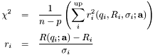
where the sum is over the data points $(q_i,R_i,\sigma_i)$ , $n$ is the number of data points, and $p$ the total number of parameters.

The mehtods employed by yanera include all those available to the GSL as well as an optional two more. In every case except NMSIMPLEX, it is possbile to hold any parameter value fixed. However, only with certain methods is it possible to constrain variables to be within certain minimum and maximum values.

The methods can be broken down into three catagories: non-linear least squares, multidimensional minimization, and simulated annealing. Also, the first two methods have constrained and uncontrained options.

Non-linear least squares

Non-linear least squares The Levenberg-Marquardt algorithm is an iterative procedure that provides a numerical solution to non-linear least squares fitting. Please refer to the Wikipedia article on the Levenberg-Marquardt algorithm for more information. (http://en.wikipedia.org/wiki/Levenberg-Marquardt_algorithm)

Implemented here are those Levenberg-Marquardt algorthims from the GSL, which are unconstrained in the library, or with naive constraints appplied. A robust Levenberg-Marquardt algotirhtm with parameter constraints comes form the levmar library.

LMSDR - unconstrained, GSL
LMDR - unconstrained, GSL
CLMSDR - constrained, GSL
CLMDR - constrained, GSL
LEVMAR - constrained, LEVMAR library (Optional for Linux version, Standard with Windows version)

The iterations can be stopped by an error, or by successful completion. For the GSL Levenberg-Marquardt algorthims, there are two stopping criterion, and the iteration stops on the success of either one. The first is when the gradient falls below a tolerance level. The test can be summarized as,

$\left|\frac{\partial\chi^2}{\partial a_i}\right| \leq \epsilon.$

The second stop test compares the residuals, $r$ , of the last step with the residuals of the current step according to,

$|r^{i-1}| \leq \epsilon_{\mathrm{absolute}} + \epsilon_{\mathrm{relative}}|r^i|$

Perhaps a later version will allow user configuration of the tolerances.

Performance

Generally, Levenberg-Marquardt algorithms are fast and robust for the common layered model types. However, when using function, or component models, since the algorithm requires calculating the gradient of $\chi^2$ with respect to $\mathbf{a}=[a_1, a_2, \ldots]$ , and these models require adaptive quadrature, this method can be slowed down.

Multidimensional minimization

Multi-dimensional minimization is a collection of iterative algorithms for finding minima of arbitrary functions. In this case, we are minimizing the Chi squared measure of the fit for a given set of parameters. All algorithms are either some form of the conjugate gradient or steepest descent methods, and numerically calculate the gradient of $\chi^2$ with respect to the parameters to choose the direction of minimization.

Implemented here are those minimization algorthims from the GSL, which are unconstrained. Optional constrained algotirhtms comes form the ool library. As implimented, it is not exactly correct, since $p$ in the equation for $\chi^2$ above should be the number of parameters not being held fixed.

CONJUGATE_FR - unconstrained conjugate gradient, GSL
CONJUGATE_PR - unconstrained conjugate gradient, GSL
VECTOR_BFGS - unconstrained conjugate gradient, GSL
STEEP_DESC - unconstrained steepest descent, GSL
NMSIMPLEX - unconstrained steepest descent without gradients, GSL
OOL_SPG - constrained steepest descent, optional OOL library, Linux only
OOL_GENCAN - constrained steepest descent, optional OOL library, Linux only

The iteration can be stopped by an error, or by successful completion. The stopping criterion is the gradient falls below a tolerance level. The test can be summarized as,

$\left|\frac{\partial\chi^2}{\partial a_i}\right| \leq \epsilon$

Performance

Generally, VECTOR_BFGS is the better of the minimizations, but is unconstrained. The NMSIMPLEX method does not suffer from speed performances because it soes not calculate the gradient. Thus it convereges very well, but very slowly, and is impoosible to fix paramters. OOL_GENCAN is better than OOL_SPG, but is much slower per iteration.

Simulated Annealing

Simulated annealing is a generic probabilistic algorithm for global optimization of a function in a large search space. In this case, we are optimizing the Chi squared measure of the fit for a given set of parameters. The search space is the space of possible parameter values. The simulated annealing routine here is implemented using the GNU Scientific Library. Please refer to the Wikipedia article on simulated annealing for more information. (http://en.wikipedia.org/wiki/Simulated_annealing)

The method here comes from the GSL, but it is always constrained.

SIMAN - constrained simulated annealing, GSL

When using this technique, it can be useful to direct the printout to be saved in a file. It will contain the system energy and parameter values over the course of the simulation, which can be analyzed later.

The initial temperature is set to be four times initial energy, which is just $\chi^2$ evaluated with the initial parameters, where $\chi^2$ is given above. The final temperature is $10^6$ times smaller. This works well when the Boltzmann constant is set to 1.

The difficulty is choosing the best step size, since there is only one that must be shared among all the variables. When the SLD and background is given in the scale of $10^{-6}$ , then all variables hopefully are of the similar order of magnitude, and can be varied by a similar step size.

Performance

The rate of convergence to a solution is highly probablistic. So it is impossible to say whether it will converge to a local or global mimimum for a given number of iterations.