MATH 6.4: Waves and partial differential equations |
PPLATO @ | |||||
PPLATO / FLAP (Flexible Learning Approach To Physics) |
||||||
|
1 Opening items
1.1 Module introduction
The purpose of this module is to provide an introduction to two topics: waves and partial differentiation. Waves occur in many physical situations, including vibrating strings, ripples on the surface of a lake, sound waves, electromagnetic radiation and so on. The study of waves will lead us to functions of two variables (in this case position x and time t) and to the derivatives of such functions. Functions of more than one variable are common throughout physics and finding the derivatives of such functions requires a knowledge of partial differentiation.
The structure of this module is as follows. In Subsection 2.1 we consider oscillations and the differential equation of simple harmonic motion (SHM). Subsection 2.2 introduces waves and draws your attention to the distinction between waves and oscillations. In Subsection 2.3 we consider functions of two variables and such functions are used in the Subsection 2.4 to describe a general wave which propagates without changing its shape. Subsection 2.5Subsections 2.5 and Subsection 2.62.6 introduce first– and second–order partial derivatives, respectively. (The techniques given here have wide applicability throughout physics and not just to the study of waves.) Subsection 2.7 derives the partial differential equation for a wave propagating in one dimension without changing its shape, and Subsection 2.8 shows how such a wave equation arises in the study of waves on a string. Subsection 2.9 shows how standing waves can occur on a vibrating string with fixed ends. Section 3 is devoted to the time-dependent and time-independent Schrödinger equations that arise in quantum mechanics. It explains the relationship between these two equations, describes the significance of some of their ‘wave-like’ solutions (called wave functions), and demonstrates the crucial role of partial derivatives in quantum mechanics.
Study comment Having read the introduction you may feel that you are already familiar with the material covered by this module and that you do not need to study it. If so, try the following Fast track questions. If not, proceed directly to the Subsection 1.3Ready to study? Subsection.
1.2 Fast track questions
Study comment Can you answer the following Fast track questions? If you answer the questions successfully you need only glance through the module before looking at the Subsection 4.1Module summary and the Subsection 4.2Achievements. If you are sure that you can meet each of these achievements, try the Subsection 4.3Exit test. If you have difficulty with only one or two of the questions, you should follow the guidance given in the answers and read the relevant parts of the module. However, if you have difficulty with more than two of the Exit questions you are strongly advised to study the whole module.
Question F1
The functions F1(x, y) and F2(x, y) are defined by
$F_1(x,\,y) = -\dfrac{\partial \phi(x,\,y)}{\partial x}\quad\text{and}\quad F_2(x,\,y) = -\dfrac{\partial \phi(x,\,y)}{\partial y}$
where $\phi(x,\,y) = \dfrac{q}{4\pi\varepsilon_0\sqrt{x^2+y^2}}$ i
Find $\sqrt{\smash[b]{F_1^2+F_2^2}}$.
Answer F1
Since
$F_1 = -\dfrac{\partial \phi}{\partial x} = -\dfrac{q}{4\pi\varepsilon_0}\dfrac{\partial}{\partial x}(x^2 + y^2)^{-1/2} = \dfrac{q}{4\pi\varepsilon_0}\dfrac{x}{(x^2 + y^2)^{3/2}}$
and
$F_2 = -\dfrac{\partial \phi}{\partial y} = -\dfrac{q}{4\pi\varepsilon_0}\dfrac{\partial}{\partial y}(x^2 + y^2)^{-1/2} = \dfrac{q}{4\pi\varepsilon_0}\dfrac{y}{(x^2 + y^2)^{3/2}}$
we obtain
$\sqrt{\smash[b]{F_1^2+F_2^2}} = \dfrac{q}{4\pi\varepsilon_0}\dfrac{(x^2 + y^2)^{1/2}}{(x^2 + y^2)^{3/2}} = \dfrac{q}{4\pi\varepsilon_0(x^2 + y^2)}$
(The electrostatic potential for a line of charge has the form given for ϕ (x, y), in which case $\sqrt{\smash[b]{F_1^2+F_2^2}}$ represents the magnitude of the electrostatic field.)
Question F2
Show that f (x − vt) is a solution of the wave equation
$\dfrac{\partial^2f}{\partial x^2} - \dfrac{1}{v^2}\dfrac{\partial^2f}{\partial t^2} = 0$
Answer F2
$\dfrac{\partial f}{\partial x} = f'(x-vt)\quad\text{and}\quad\dfrac{\partial^2f}{\partial x^2} = f''(x-vt)$
Also
$\dfrac{\partial f}{\partial t} = -vf'(x-vt)\quad\text{and}\quad\dfrac{\partial^2f}{\partial t^2} = v^2f''(x-vt)$
and the required result follows immediately.
Question F3
The one–dimensional time–dependent Schrödinger equation for a particle of mass m with a potential energy function U (x, t) is
$-\dfrac{\hbar^2}{2m}\dfrac{\partial^2{\it\Psi}(x,\,t)}{\partial x^2} + U(x,\,t){\it\Psi}(x,\,t) = i\hbar\dfrac{\partial{\it\Psi}(x,\,t)}{dt}$
Show that ${\it\Psi}(x,\,t) = \exp(-m\omega x^2/(2\hbar))\exp(-iEt/\hbar)$ i
is a solution of this equation with $U(x,\,t) = \dfrac{m\omega^2x^2}{2}$ where ω is a constant (so that U is a function of the single variable x), and find an expression for E in terms of ω.
Answer F3
$\dfrac{\partial{\it\Psi}}{\partial x} = -\dfrac{m\omega}{\hbar} x\exp\left(-\dfrac{m\omega}{2\hbar}x^2\right)\exp\left(-i\dfrac{Et}{\hbar}\right)$
Differentiating again with respect to x we obtain
$\dfrac{\partial^2{\it\Psi}}{\partial x^2} = \left[-\dfrac{m\omega}{\hbar} + \left(\dfrac{m\omega x}{\hbar}\right)^2\right]\exp\left(-\dfrac{m\omega}{2\hbar}x^2\right)\exp\left(-i\dfrac{Et}{\hbar}\right)$
and substituting in the left–hand side of the time–dependent Schrödinger equation we have
$\left\{-\dfrac{\hbar^2}{2m}\left[-\dfrac{m\omega}{\hbar} + \left(\dfrac{m\omega x}{\hbar}\right)^2\right] + \dfrac{m\omega^2x^2}{2}\right\} \times \exp\left(-\dfrac{m\omega}{2\hbar}x^2\right)\exp\left(-i\dfrac{Et}{\hbar}\right) = \dfrac{\hbar\omega}{2}\exp\left(-\dfrac{m\omega}{2\hbar}x^2\right)\exp\left(-i\dfrac{Et}{\hbar}\right)$
Differentiating Ψ with respect to t we obtain
$\dfrac{\partial{\it\Psi}}{\partial t} = -\dfrac{iE}{\hbar}\exp\left(-\dfrac{m\omega}{2\hbar}x^2\right)\exp\left(-i\dfrac{Et}{\hbar}\right)$
and therefore the right–hand side of the time–dependent Schrödinger equation can be written as
$E\exp\left(-\dfrac{m\omega}{2\hbar}x^2\right)\exp\left(-i\dfrac{Et}{\hbar}\right)$
which means that the expression given for Ψ is a solution provided that $E = \dfrac{\hbar\omega}{2}$.
The particular form of U given in this question is the potential energy function for a simple harmonic oscillator, and E is the lowest energy level for the quantum mechanical version of such an oscillator. Notice that E is not zero, even for the lowest energy state.
1.3 Ready to study?
Study comment To begin the study of this module you need to be familiar with the following topics: the trigonometric functions and trigonometric identities (specific identities will be supplied when needed); Cartesian coordinates and graph sketching (including the concept of a tangent_to_a_curvetangent to a graph, and the determination of the gradient of a straight line); the differentiation of functions of one variable (including the definition of a derivative in terms of a limit and the rules of differentiation, particularly the chain rule); the derivatives of the trigonometric_functionstrigonometric and exponential functions, polynomial_functionpolynomials and power_mathematicalpowers; differential equations (including the role of boundary conditions in determining a solution_mathematicalsolution to such an equation), and for Section 3, the properties of complex numbers (including the rules for their addition and multiplication, and the meaning of the modulus of a complex number). You need to have some acquaintance with the basic ideas of Newtonian mechanics, including energy, momentum, power and Newton’s laws of motion; it would also be useful to have had some previous experience of waves (including their wavelength, frequency and speed) since this module only provides a brief review of their properties. In a similar spirit it would be helpful, but not essential, to have some knowledge of simple harmonic motion, and Hooke’s law. Finally, you will also need to have some idea of the everyday meaning of the term probability, though you are not expected to be familiar with any of the mathematical properties of probability. The following questions will help you to establish whether you need to review some of the above topics before embarking on this module.
Question R1
Differentiate the following functions with respect to x:
(a) f (x) = 3x2 + 4x5
(b) g (x) = exp(λx3), where λ is a constant,
(c) h (x) = cos(x + 3x3)
(d) $w(x) = \dfrac{x+1}{x^2+2}$
(e) u (x) = (x2 + c2)2, where c is a constant
(f) v (x) = [x2 + sin(yx)]3, where y is a constant,
(g) p (x) = sin(ax − bt), where a, b and t are constants.
Answer R1
(a) Using $\dfrac{d(x^n)}{dx} = nx^{n-1}$ we get
$\dfrac{df(x)}{dx} = 6x + 20x^4$
(b) Since $\dfrac{d(\exp(ax))}{dx} = a\exp(ax)$ we have
$\dfrac{dg(x)}{dx} = 3x^2\lambda\exp(\lambda x^3)$
(Remember that exp(λx3) is merely an alternative way of writing eλx3. When we use this alternative notation in this module we do so principally because the superscripts are otherwise rather small.)
(c) Using the standard derivative $\dfrac{d\cos(x)}{dx} = -\sin(x)$ and the chain rule we obtain
$\dfrac{dh(x)}{dx} = -(1 + 9x^2)\sin(x+3x^3)$
(d) If u and v are functions of x, we have
$\dfrac{d}{dx}\left(\dfrac uv\right) = \left.\left(v\dfrac{du}{dx} - u\dfrac{dv}{dx}\right)\middle/v^2\right.$
(the quotient_rule_of_differentiationquotient rule) so that
$\dfrac{dw(x)}{dx} = \dfrac{1}{(x^2+2)^2}\left[(x^2+2)-(x+1)(2x)\right] = -\dfrac{x^2-2x+2}{(x^2+2)^2}$
(e) $\dfrac{du}{dx} = 2(x^2+ c^2) \times 2x = 4x(x^2+c^2)$ from the chain rule.
(f) $\dfrac{dv}{dx} = 3(x^2+ \sin(yx))^2(2x + y\cos(yx))$ again from the chain rule.
(g) $\dfrac{dp}{dx} = a\cos(ax-bt)$
Question R2
Show that:
(a) if k is an arbitrary constant, $y(x) = \dfrac{x^3}{6} + \dfrac{k}{x^3}$ is a solution of the differential equation $\dfrac{dy}{dx} + \dfrac{3y}{x} = x^2$.
(b) if a and b are arbitrary constants, y (x) = a e−x + b e−2x is a solution of the differential equation $\dfrac{d^2y}{dx^2} + 3\dfrac{dy}{dx} + 2y = 0$.
Answer R2
(a) Differentiating y (x) we have $\dfrac{dy}{dx} = \dfrac{x^2}{2} -\dfrac{3k}{x^4}$, which can be substituted into the left–hand side of the differential equation, giving $\left(\dfrac{x^2}{2} - \dfrac{3k}{x^4}\right) + \dfrac 3x \left(\dfrac{x^3}{6} + \dfrac{k}{x^3}\right)$ which simplifies to give x2. Since this is equal to the right–hand side of the given equation, we have verified that y (x) is a solution of the differential equation.
(b) Differentiating y (x) once with respect to x we get $\dfrac{dy}{dx} = -a{\rm e}^{-x} - 2b{\rm e}^{-2x}$ and differentiating again gives $\dfrac{d^2y}{dx^2} = a{\rm e}^{-x} + 4b{\rm e}^{-2x}$.
Substituting these results into the left–hand side of the differential equation, we obtain
$\dfrac{d^2y}{dx^2} +3\dfrac{dy}{dx} +2y = \left(a{\rm e}^{-x} + 4b{\rm e}^{-2x}\right) + 3\left(a{\rm e}^{-x} + 4b{\rm e}^{-2x}\right) + 2\left(a{\rm e}^{-x} + b{\rm e}^{-2x}\right)$
$\phantom{\dfrac{d^2y}{dx^2} +3\dfrac{dy}{dx} +2y }= a{\rm e}^{-x}(1-3+2) + b{\rm e}^{-2x}(4-6+2) = 0$
which verifies that y (x) is a solution.
Question R3
(a) Evaluate the limit $\displaystyle \lim_{\Delta x\rightarrow 0}{\left[\dfrac{(a + \Delta x)^2 - a^2}{\Delta x}\right]}$. What does this limit represent?
(b) If y = f (x) then the derivative $\dfrac{dy}{x}$ is sometimes written alternatively as f ′ (x).
What does the limit $\displaystyle \lim_{\Delta x\rightarrow 0}{\left[\dfrac{f '(x+\Delta x) - f'(x)}{\Delta x}\right]}$ represent?
Answer R3
(a) $\displaystyle \lim_{\Delta x\rightarrow 0}\left[\dfrac{(a + \Delta x)^2- a^2}{\Delta x}\right] = \lim_{\Delta x\rightarrow 0}\left[\dfrac{2a\Delta x + (\Delta x)^2}{\Delta x}\right] = \lim_{\Delta x\rightarrow 0}(2a + ∆x) = 2a$.
If y = f (x) = x2 then the limit represents $\dfrac{dy}{dx}$ evaluated at x = a, which can be written as f ′ (a).
(b) The limit represents $\dfrac{d^2y}{dx^2}$, the second derivative of y with respect to x, which is sometimes alternatively written as f ′′ (x).
Comment If you had difficulty with any of the Ready to study questions, consult the relevant entries in the Glossary.
2 Waves and oscillations
2.1 Oscillations
An oscillation is said to occur when some quantity (such as position) repeatedly cycles about an equilibrium value.
Although oscillations are often taken to be sinusoidal i (see Figure 1), this is not necessarily the case and other forms (which arise, for example, in the context of electric circuits) are shown in Figure 2 and Figure 3.
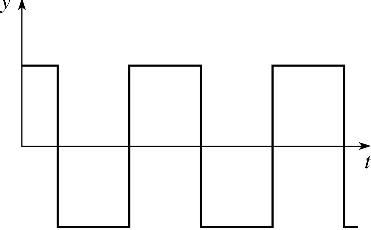
Figure 3 Square–wave oscillation.
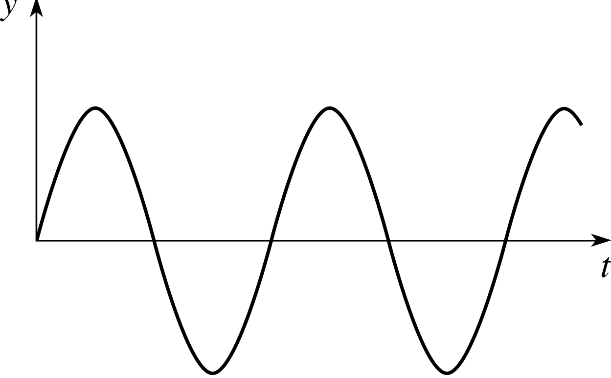
Figure 1 Sinusoidal oscillation.
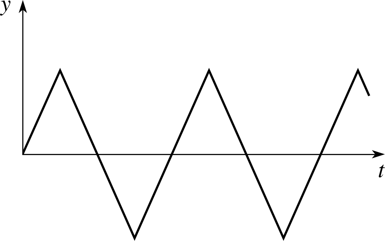
Figure 2 Triangular oscillation.
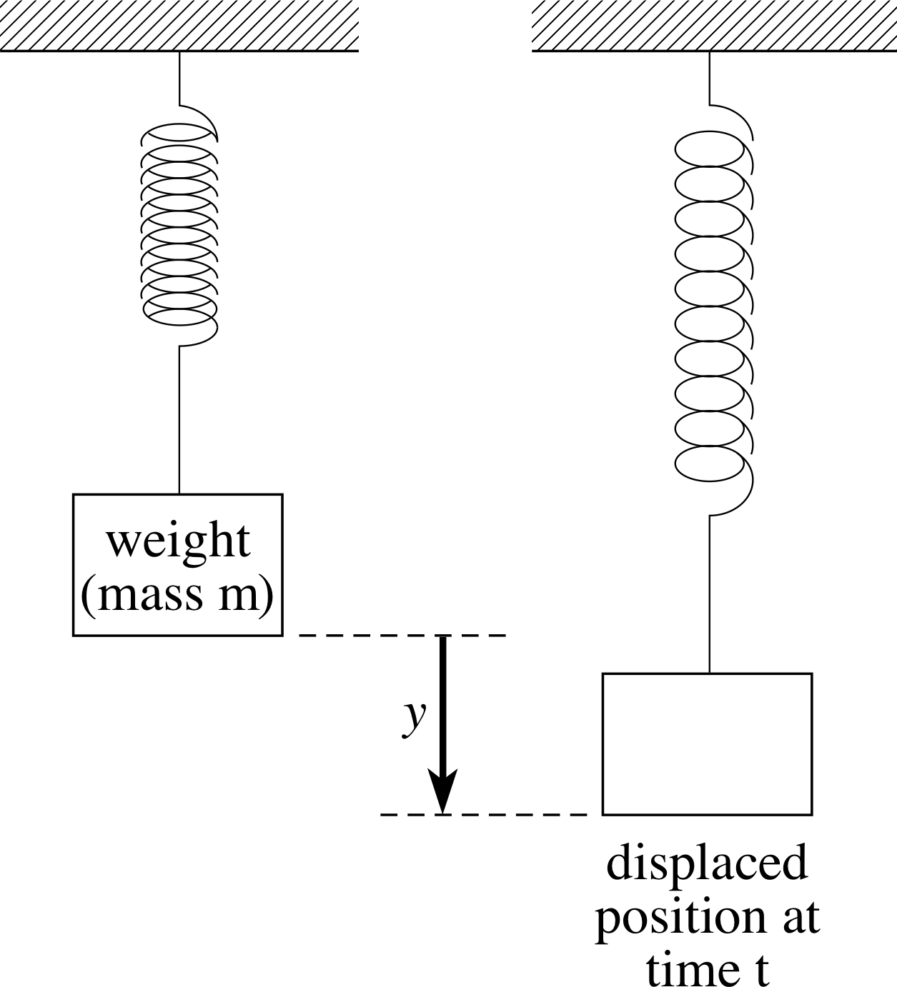
Figure 4 An oscillating system; a mass on a spring.
A typical physical example of an oscillating system is a mass on a spring after the mass has been displaced from its equilibrium position and released (as in Figure 4). After its release, the displacement of such a mass exhibits an approximately sinusoidal oscillation similar to that in Figure 1. Hooke’s law is often used to provide a mathematical model of a spring, and using it we can derive an equation which describes the motion of the mass. So–called ‘ideal springs’, which satisfy Hooke’s law, have the property that the extension of the spring y, is proportional to the restoring force Fy that causes the mass to return towards its equilibrium position. Thus, for such a spring
Fy = −ky(1)
where k is a (positive) constant.
If m is the mass, then Newton’s second law allows us to replace Fy by $m\dfrac{d^2y(t)}{dt^2}$, which shows that y (t) satisfies
$m\dfrac{d^2y(t)}{dt^2} = -ky(t)$(2)
If we introduce the positive constant ω defined by $\omega = \sqrt{k/m\os}$ we may rewrite Equation 2 in the form
$\dfrac{d^2y(t)}{dt^2} = -\omega^2y(t)$(3)
Equation 3 is a differential equation. It can be solved for y (t), and the general solution is
y (t) = A sin(ωt) + B cos(ωt)(4)
where A and B are arbitrary constants. This general solution can also be written in the alternative (and often more useful form)
y (t) = C sin(ωt + ϕ)(5)
where C and ϕ are arbitrary constants, and we still have $\omega = \sqrt{k/m\os}$.
Equation 5 is an especially valuable form of the solution because it makes it easy to identify the physical significance of each of the terms:
C is the amplitude and represents the maximum value of the displacement from the equilibrium position; (ωt + ϕ) is called the phase and determines the stage that the oscillation has reached in its cycle at time t;
$\omega = \sqrt{k/m\os}$ is called the angular frequency and is 2π times the number of oscillations completed per second;
andϕ is called the phase constant (or the initial phase) since it determines the value of the phase at t = 0, and hence the displacement from equilibrium at that time (y (0) = C sin ϕ).
The sort of oscillatory motion described by Equation 5, and characterized by the parameters C, ω and ϕ, is known as simple harmonic motion.
✦ Show that y (t) = C sin(ωt + ϕ) is a solution of the differential equation $\dfrac{d^2y(t)}{dt^2} = -\omega^2y(t)$
✧ Using the standard results
$\dfrac{d}{dx}\sin x = \cos x\quad\text{and}\quad\dfrac{d}{dx}\cos x = -\sin x$
we have $\dfrac{dy}{dt} = C\omega\cos(\omega t + \phi)$
and therefore
$\dfrac{d^2y}{dt^2} = -C\omega^2\sin(\omega t + \phi) = -\omega^2y(t)$
Other examples of physical systems which display oscillatory behaviour include the simple pendulum and some a.c. circuits, but the basic idea remains the same; some physical quantity, for example position, voltage or current, cycles repeatedly about an equilibrium value.
2.2 Waves
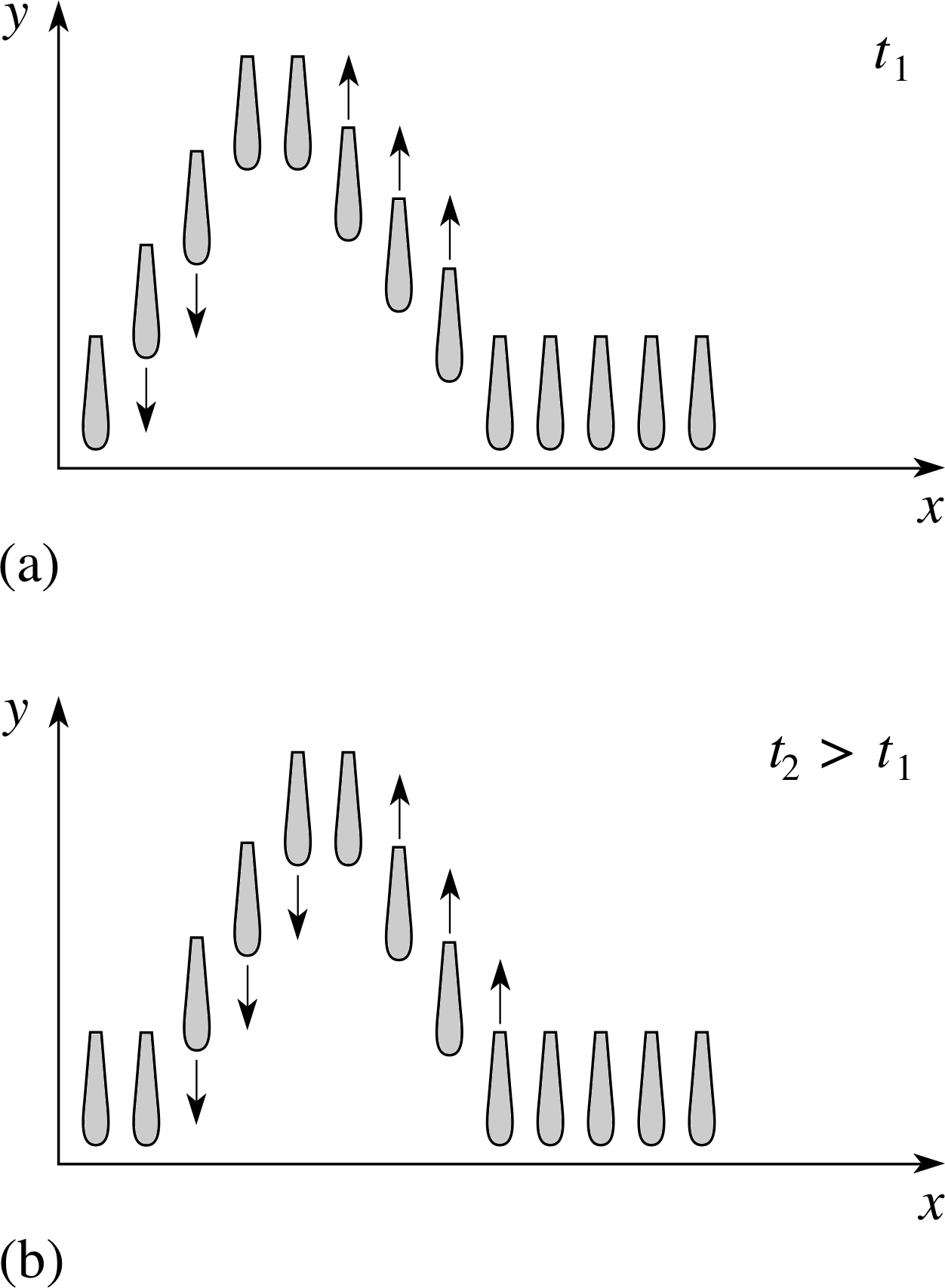
Figure 5 Snapshots at two different times of the heights of all the hammers in a piano show how vertical movements can produce a wave that travels horizontally. Notice particularly that the vertical displacement y at any position x (measured from the left–hand end of the keyboard) is dependent on two factors: the particular hammer and the time, i.e. the value of x and the value of t. The time t2 in (b) is later than t1 in (a).
Perhaps the first thing that comes to mind when you see the word ‘wave’ is the wave that you see at the beach. The undulations of the surface of the sea occur in a regular fashion, and appear to move towards the shore – a phenomenon that surfers are able to exploit to the full. We say that the surface ‘appears to move’ because the actual motion of the water is a good deal more complicated than you would at first think. Clearly something moves towards the shore, but it is certainly not a coherent body of water, for otherwise the entire ocean would end up on the beach. As further evidence of this you need only note that a swimmer tends to bob up and down as a wave passes, and this would certainly not happen if the velocity of the water at each point in the wave was directed towards the shore.
There is a well known Tom and Jerry cartoon that illustrates what is really happening. Tom is seated at a grand piano and runs his thumb rapidly along the keys from left to right, while Jerry is inside the piano and moves along with the wave of displaced hammers (see Figure 5). The essential point to appreciate is that the hammers are simply moving up and down, while the wave moves from left to right. The wave is a travelling disturbance in the position of each hammer, not a travelling set of hammers.
A water wave is a very similar phenomenon. The motion of the water is predominantly vertical and oscillatory, while the motion of the wave is horizontal and progressive.
Another place where we are used to seeing waves is on strings, ropes and cables. These waves take many forms. For instance, if you hold one end of a long string and give it a single flick, then a solitary wave (often referred to as a pulse) will travel along the string. On the other hand if you jerk the string up and down repeatedly in a regular way, you may produce a repetitive wave that travels along the string. Note that the disturbance does not have to be repetitive in order to qualify as a wave. Both kinds of disturbance travel along the string, so both are examples of travelling waves.
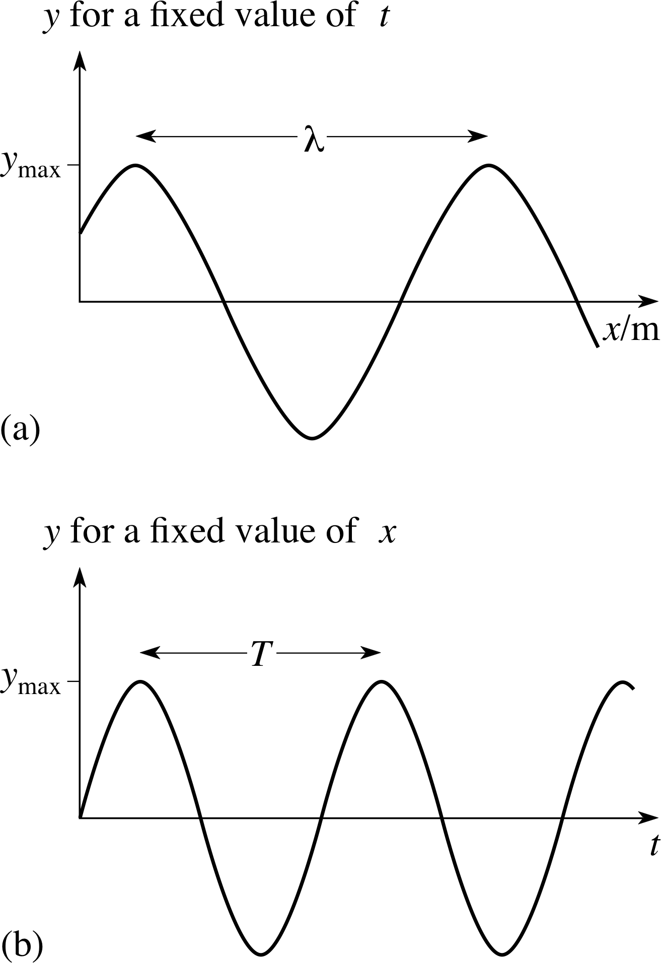
Figure 6 (a) The ‘shape’ of a sinusoidal travelling wave at a particular instant of time – the wave profile. (b) The oscillation caused by a sinusoidal travelling wave at a particular point – the wave form.
Although travelling waves do not have to be repetitive, there can be no doubt that the best known and most intensively studied kind of travelling wave is one which has a sinusoidal shape at each successive instant of time. Figure 6 attempts to illustrate such a sinusoidal wave, such as one travelling along a string. As you can see, the figure is in two parts. Figure 6a shows the displacement y at all points x at a fixed time t; in effect, this is a ‘snapshot’ of the wave. Figure 6b, on the other hand, shows the way in which the displacement y changes with time at a fixed position x. If you compare Figure 6b with Figure 1 you will see that at a fixed value of x the disturbance caused by the sinusoidal travelling wave is just a sinusoidal oscillation. Indeed, one way of picturing a sinusoidal travelling wave is as an array of simple harmonic oscillators, where each oscillator is slightly out of phase, i.e. has a slightly different initial phase compared with its neighbours.
A ‘snapshot’ of a wave at a particular instant, such as Figure 6a, is generally referred to as a wave profile. A trace showing the changing disturbance caused by a wave at a fixed point, such as Figure 6b is called a wave form. Both of these terms will be used freely in the rest of this module. Remembering that both are needed to characterize a wave will help you to remember the distinction between a wave and an oscillation. If you were to photograph a travelling wave on a string you would obtain a wave profile. To determine the wave form you would have to record the displacement of a particular segment of string at different times.
The need for both a wave profile and a wave form in order to characterize a wave points to the essential mathematical difference between a wave and an oscillation. In the case of an oscillating mass, the displacement from the equilibrium position y, is only a function of time; so it may be represented by y (t). On the other hand, for a wave on a string the displacement from the equilibrium position is a function of position and time; so it may be represented by y (x, t). Thus, even when it only travels in one dimension (x), the wave disturbance y is a function of two variables. We shall consider such functions in more detail in Subsection 2.3, but first we shall finish this subsection by briefly introducing some of the parameters commonly used to describe waves.
If we stay with our example of a wave on a string, then the amplitude A is the maximum displacement (in the y–direction) of the string from its equilibrium position. The wavelength λ is the distance between two successive peaks (or troughs) on the wave profile, as shown in Figure 6a. i One might determine the wavelength by photographing the string, and then measuring the distance between the peaks. The period T is the time between two successive peaks (or troughs) on the wave form as shown in Figure 6b, and this might be found by timing the interval between peaks at a fixed position on the string. The frequency f is the number of troughs (or peaks) which pass a fixed location in one second, and is related to the period by
$f = \dfrac 1T$(6)
The units of frequency will therefore be s−1, which are called hertz (Hz) in SI units. Since f is the rate at which peaks pass a fixed point, and since the distance between successive peaks is λ, it follows that the speed of propagation v at which the waves move along the string is given by
v = f λ(7)
The angular frequency ω is related to the period by the equation
$\omega = 2\pi f = \dfrac{2\pi}{T}$(8)
so ω = 2πf, and ω is in units of rad s−1.
Similarly, the wavenumber σ and the angular wavenumber k are related to the wavelength λ by the equations
$\sigma = \dfrac{1}{\lambda}$(9)
and$k = \dfrac{2\pi}{\lambda}$(10) i
It is probably worthwhile to try to remember Equations 6 to 10, since there are many useful relationships that can be derived from them. The basic definitions are summarized in Table 1.
| Amplitude | A | The maximum displacement from equilibrium, see Figure 6a or 6b. | ||
|---|---|---|---|---|
| Wavelength | λ | The distance that separates adjacent equivalent points on the wave profile, see Figure 6a. | ||
| Period | T | The time that separates successive equivalent points on the wave form, see Figure 6b. | ||
| Frequency | f | = 1/T | ||
| Angular frequency | ω | = 2πf = 2π/T | ||
| Wavenumber | σ | = 1/λ | ||
| Angular wavenumber | k | = 2π/λ | ||
| Speed of propagation | v | = f λ = ω/k |
✦ Use the definitions that have been presented to show that v = ω/k.
✧ From Equations 7 and 8
v = f λ(Eqn 7)
$\omega = 2\pi f = \dfrac{2\pi}{T}$(Eqn 8)
we have
$v = f\lambda = \dfrac{\omega}{2\pi} \times \lambda = \dfrac{\omega}{k}$
Figure 6 (a) The ‘shape’ of a sinusoidal travelling wave at a particular instant of time – the wave profile. (b) The oscillation caused by a sinusoidal travelling wave at a particular point – the wave form.
Waves which cause a disturbance perpendicular to their direction of propagation are known as transverse waves. Waves on a string, ripples on a pond and electromagnetic waves are all examples of transverse waves, but not all waves are transverse.
Sound waves in air are caused by compression and rarefaction of the atmosphere as molecules move back and forth along the direction of propagation. Such waves are known as longitudinal waves. For a sound wave, we can still represent the displacement from the equilibrium position by y and draw graphs similar to Figure 6, but x and y are not physically perpendicular in that case.
2.3 Functions of two variables
As we have seen, if y is the displacement from the equilibrium position for a one-dimensional wave, then y is a function of two variables, the position x, and the time t. In order to emphasize that y is a function of both x and t we may write it as y (x, t). Here is an example of such a function:
y (x, t) = A sin(at − bx)(11) i
where A = 2.37 m, a = 16 s−1, and b = 3.23 m−1. Note that the units of a and b are such that when we substitute values for t and x (in seconds and metres respectively) the argument of the sine function will be dimensionless, as it should be.
✦ Evaluate y (1.9 m, 12.0 s) from the definition of y (x, t) given in Equation 11. i
✧ y (1.9 m, 12.0 s) = (2.37 m) × sin(16 s−1 × 12.0 s − 3.23 m−1 × 1.9 m) = (2.37 m) × (−0.487) = −1.15 m.
Functions of two variables occur quite often in physical situations, i here are some examples.
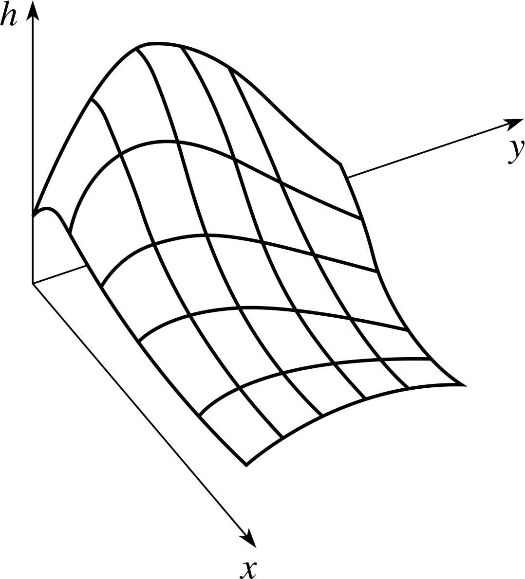
Figure 7 The height h (x, y) above the (x, y) plane.
- 1
-
Suppose we want a mathematically precise description of a hill or a mountain range. We could obtain such a description by first using a two–dimensional coordinate system to specify points on a horizontal reference surface (e.g. sea-level), and then using a function of two variables h (x, y), to represent the height of the Earth’s surface above sea–level at a point with coordinates (x, y).
A function of this kind is difficult to illustrate on a sheet of paper but a useful picture can often be obtained by means of a three–dimensional graph of the sort shown in Figure 7.
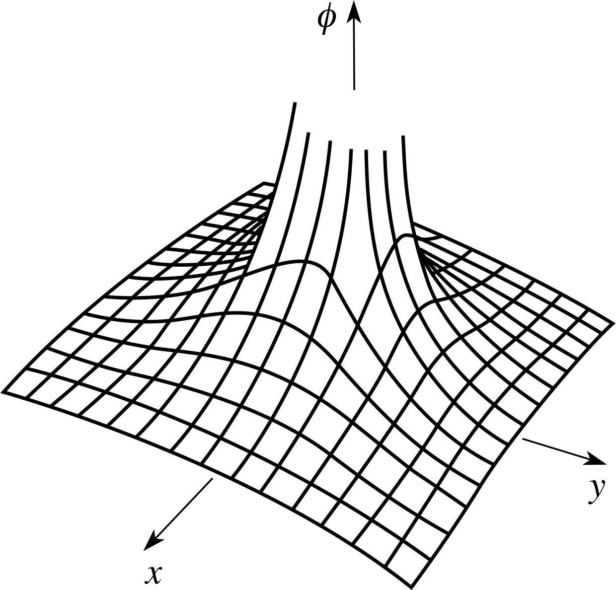
Figure 8 The function ϕ (x, y) of Equation 12.
- 2
-
If a fixed electric charge q (measured in coulombs) is located at the origin of a Cartesian coordinate system the electrostatic potential at any point in the (x, y) plane with coordinates (x, y) is given by
$\phi(x,\,y) = \dfrac{q}{4\pi\varepsilon_0\sqrt{x^2+y^2}}$(12)
where ϕ is a function of the two variables x and y, and ε0 is a constant. This function is shown in Figure 8.
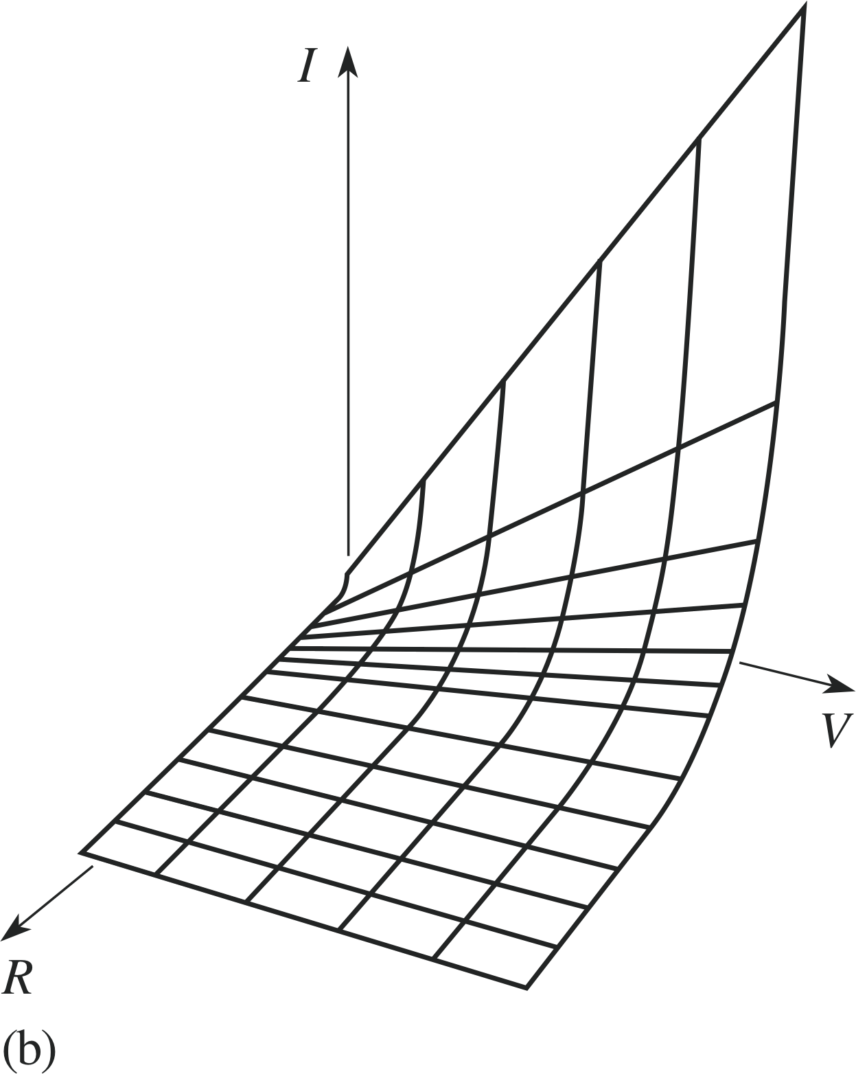
Figure 9b The current I as a function of V and R.
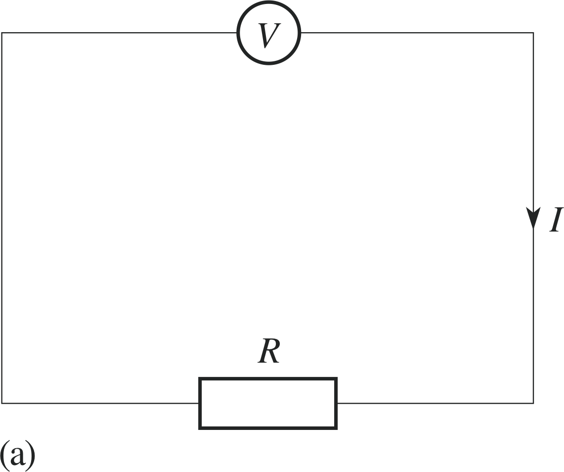
Figure 9a The current I as a function of V and R.
- 3
-
The current I, the voltage V, and the resistance R in a circuit such as that shown in Figure 9a are related by Ohm’s law
I = VR(13)
In a situation in which V and R can be varied independently, I is a function of these two variables and can be written as I (V, R). This function is shown in Figure 9b.
It is sometimes convenient to display the arguments of the same function in different ways.
For example, if ϕ (x, y) = q, as in Equation 12,
$\varphi(x,\,y) = \dfrac{q}{4\pi\varepsilon_0\sqrt{x^2+y^2}}$(Eqn 12)
then, although ϕ is a function of the two variables x and y, it can also be considered as a function of the single variable u = x2 + y2, and we can write
$\varphi(u) = \dfrac{q}{4\pi\varepsilon_0\sqrt{u\os}}$(14)
where u = x2 + y2. In such a case we may avoid having to introduce the extra variable u by writing the function ϕ
in the form
$\varphi(x^2+y^2) = \dfrac{q}{4\pi\varepsilon_0\sqrt{x^2+y^2}}$(15) i
✦ If $y(x,\,t) = \sin\left(\dfrac{2\pi}{\lambda}(x-vt)\right)$ write y as a function of a single variable.
✧ One possibility is
$y(x - vt) = \sin\left(\dfrac{2\pi}{\lambda}(x - vt)\right)$
We could of course replace x − vt by an extra variable u say, and write
$y(u) = \sin\left(\dfrac{2\pi}{\lambda}u\right)$
where u = x − vt.
You will see shortly that the above discussion is relevant to the study of waves.
2.4 The general wave
In this module we are interested in waves for which the displacement from the equilibrium position depends on the time (t) and a single space variable (x). Such waves are called one–dimensional waves, and a typical example is provided by a wave on a string of the kind we considered earlier. In general, a one–dimensional wave consists of any disturbance which moves along a line, but we are more often interested in waves which maintain their shape as they move with a constant speed. Our first example is a disturbance in the form of a parabola.
✦ Sketch the graphs of the following functions:
(a) y (x) = (x − vt)2 when t = 0 s and v = 1 m s−1
(b) y (x) = (x − vt)2 when t = 1 s and v = 1 m s−1
(c) y (x) = (x − vt)2 when t = 2 s and v = 1 m s−1
Does the ‘pulse’ move to the left or to the right as t increases? In which direction would the pulse move if (x − vt)2 was replaced by (x + vt)2?
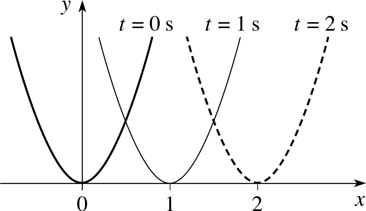
Figure 10 The graph of y (x) = (x − vt)2 for t = 0 s, 1 s and 2 s.
✧ The parabola y (x) = (x − vt)2, with v = 1 m s−1, moves to the right as t increases. The parabola y (x) = ( x + vt )2 with v = 1 m s−1, would move to the left as t increases.
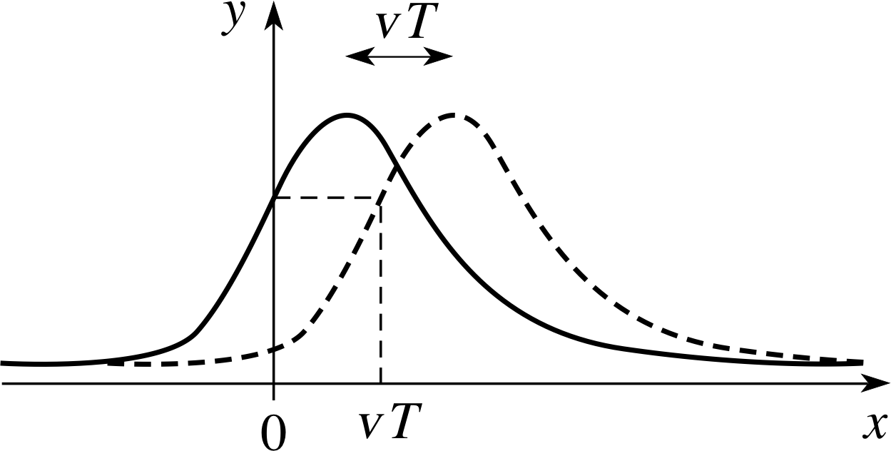
Figure 11 A general wave moving a distance vT to the right.
The continuous curve in Figure 11 shows a snapshot of a solitary wave pulse at some initial time t = 0, when it has a profile given by y = f (x). The dashed curve shows another snapshot of the same wave at a later time t = T where T > 0. If the wave moves to the right at constant speed v, without changing its shape, then during the time T that elapses between the two snapshots each part of the wave will travel a distance vT to the right. It follows that the disturbance y at any position x at time t = T will be equal to the disturbance that would have existed at x − vT at t = 0. Hence, at t = T the wave profile is given by y = f (x − vT), where f is the same function that described the wave profile at t = 0. Of course, there was nothing special about the value of T that we chose, so we can say that at any positive time t (including t = 0) any wave that moves in the positive x–direction with unchanging shape and constant speed v can be represented by
y = f (x − vt)
Similarly a wave that moves to the left with unchanging shape can be represented by
y = f (x + vt)
where y = f (x) describes the profile of the wave at t = 0.
Question T1
A function θ (x) is defined by
$\theta(x) = \cases{0 \text{ for } x \lt 0 \\ 1 \text{ for } x \ge 0}$(16)
and a function y (x, t) is defined by y (x, t) = θ (x − vt). Sketch graphs of y, as a function of x, for vt = 0 m, 1 m, 2 m. Repeat the exercise for y (x, t) = θ (x + vt).
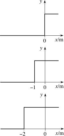
Figure 17 y (x, t) = θ (x + vt) for vt = 0 m, 1 m, 2 m.
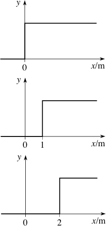
Figure 16 y (x, t) = θ (x − vt) for vt = 0 m, 1 m, 2 m.
Answer T1
See Figures 16 and 17.
To a physicist, sinusoidal waves are of paramount interest for several reasons:
- 1
-
Many waves that occur in physics are sinusoidal, including monochromatic light (i.e. of a single wavelength), sound generated by a fixed frequency oscillator and radio waves (when unmodulated by speech, etc)..
- 2
-
Sinusoidal waves are comparatively simple to analyse.
- 3
-
In most cases, a complicated wave can be considered as the sum of sinusoidal waves of different frequency.
A sinusoidal wave, moving to the right with constant speed v, as t increases, may be written in the general form
y (x, t) = A sin[k (x − vt) + ϕ](17) i
where the constants A, k and ϕ, respectively, represent the amplitude of the wave, its angular wavenumber and its phase constant.
Unless we are comparing two waves, the phase constant is of little interest and we may assume that it is zero; in which case Equation 17 may be written in any one of the following equivalent forms (using Equations 6 to 10, which are repeated for your convenience):
| y (x, t) = A sin[k (x − vt)] | (18) | $f = \dfrac 1T$ | (Eqn 6) |
| y (x, t) = A sin[kx − ωt] | (19) | v = f λ | (Eqn 7) |
| y (x, t) = A sin[2π (σx − ft)] | (20) | ω = 2π/T | (Eqn 8) |
| $y(x,\,t) = A\sin\left[2\pi\left(\dfrac{x}{\lambda}-ft\right)\right]$ | (21) | $\sigma = \dfrac{1}{\lambda}$ | (Eqn 9) |
| $y(x,\,t) = A\sin\left[2\pi\left(\dfrac{x}{\lambda}-\dfrac tT\right)\right]$ | (22) | $k = \dfrac{2\pi}{\lambda}$ | (Eqn 10) |
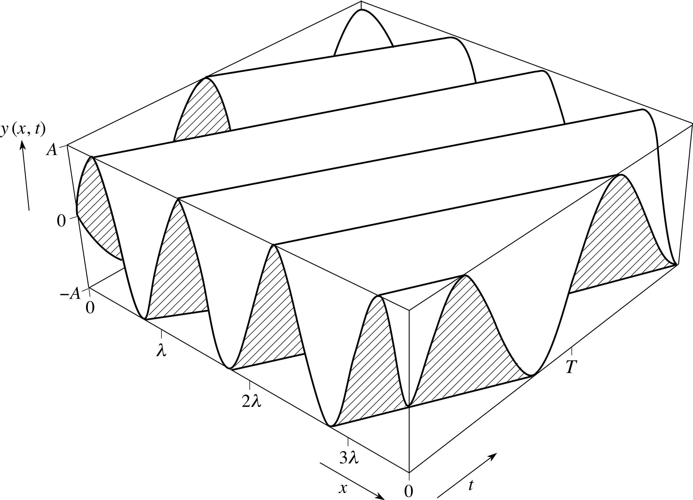
Figure 12 A three–dimensional graph of the function y (x, t) = A sin[kx − ωt].
Each of these forms has its uses, but Equation 19 is probably the most practical, and you can use Equations 6 to 10 to generate the others when you need them. Figure 12 illustrates the function given in Equation 19. Notice that each fixed value of t corresponds to a sinusoidal curve drawn on the surface. Such a curve represents the wave profile at that particular value of t (i.e. a plot of y against x at a fixed value of t). If we were to take a slightly larger fixed value of t then the wave profile would move to the right. A fixed value of x also produces a sinusoidal curve on the surface, but this time it corresponds to the wave form.
2.5 Partial derivatives
Given a function of a single variable, f (x), its rate of change at x = a is equal to the gradient of the graph y = f (x) at x = a, i and may be determined by evaluating the derivative dy/dx = f ′ (x) at x = a. The rate of change of a function of one variable is an important concept because it often arises in mathematical models of physical systems, notably in the context of differential equations.
Rates of change are also important for functions of two variables such as f (x, t), but in that context the presence of more than one independent variable introduces additional complications. Functions of two variables may have many different rates of change at a given point, and care must be taken to distinguish between them. In order to do this we need to extend the notion of an ordinary derivative to that of a partial derivative. The main purpose of this subsection is to introduce you to these partial derivatives, but before doing so we need to review the rules normally employed in the differentiation of a function of one variable.
The derivative of a function of a single variable
The rules of differentiation for a function of one variable are the following:
The constant_multiple_rule_for_differentiationconstant multiple rule:$\dfrac{d\left(cf(x)\right)}{dx} = c\dfrac{df(x)}{dx}$
The sum_rule_for_differentiationsum rule: $\dfrac{d\left(f(x)+g(x)\right)}{dx} = \dfrac{df(x)}{dx}+\dfrac{dg(x)}{dx}$
The product_rule_of_differentiationproduct rule: $\dfrac{d\left(f(x)g(x)\right)}{dx} = f(x)\dfrac{dg(x)}{dx}+g(x)\dfrac{df(x)}{dx}$
The quotient_rule_of_differentiationquotient rule: $\dfrac{d}{dx}\left(\dfrac{f(x)}{g(x)}\right) = \dfrac{g(x)df/dx - f(x)dg/dx}{\left[g(x)\right]^2}$
The chain rule: $\dfrac{df \left(u(x)\right)}{dx} = \dfrac{df(u)}{du}\dfrac{du(x)}{dx}$
As an example of the chain rule, suppose that we are given a function f (u) and that we wish to differentiate y = f (x2 + 3x) with respect to x.
Using the chain rule we can write
$\dfrac{dy}{dx} = \dfrac{df}{du}\dfrac{du}{dx}$
where u = x2 + 3x, and this gives
$\dfrac{dy}{dx} = \dfrac{df}{du}\dfrac{du}{dx} = (2x+3)\left.\dfrac{df}{du}\,\right\rvert_{u=x^2+3x}$(23)
where the final term on the right means that $\dfrac{df}{du}$ must be evaluated for u = x2 + 3x.
The notation on the right of Equation 23 is rather cumbersome, and it is often preferable to use the notation f ′ (u) in place of $\dfrac{df}{du}$, in which case Equation 23 becomes
$\dfrac{dy}{dx} = \dfrac{df}{du}\dfrac{du}{dx} = (2x+3)f'(x^2+3x)$(24)
Notice that this notation also has the advantage that we can avoid introducing the unnecessary variable u. A more general statement of this form of the chain rule then becomes
$\dfrac{d}{dx}f\left(g(x)\right) = g'(x)f'\left(g(x)\right)$(25)
(In the example above, g (x) = x2 + 3x becomes, in this notation, g ′ (x) = 2x + 3).
✦ Using the chain rule, write down the derivative with respect to x of each of the following functions:
(a) y = sin(3x + 5)
(b) y = sin(ax + b) where a and b are constants
(c) y = sin(kx − ωt) where k, ω and t are constants
(d) y = f (3x + 5) where f (u) is an arbitrary function
✧ (a) $\dfrac{dy}{dx} = 3\cos(3x+5)$
(b) $\dfrac{dy}{dx} = a\cos(ax+b)$
(c) $\dfrac{dy}{dx} = k\cos(kx-\omega t)$
(d) $\dfrac{dy}{dx} = \left.3\dfrac{df}{du}\,\right\rvert_{u = 3x+5}$
✦ (a) Given that f (x) = (x2 + 5x + 2)3 write down an expression for f ′ (x).
(b) Given that ϕ (t) = cos(at + b) where a and b are constants, write down an expression for ϕ ′ (t).
✧ (a) f ′ (x) = 3 (x2 + 5x + 2)2 (2x+5)
(b) ϕ ′ (t) = −a sin(at + b)
✦ (a) Given that y = f (kx − ωt) where k, ω and t are constants, write $\dfrac{dy}{dx}$ in terms of f ′.
(b) Given that y = f (kx − ωt) where k, ω and x are constants, write $\dfrac{dy}{dx}$ in terms of f ′.
✧ (a) $\dfrac{dy}{dx} = kf'(kx - \omega t)$
(b) $\dfrac{dy}{dt} = -\omega f'(kx-\omega t)$
The derivatives of a function of two variables
The last question, in which first x and then t was a constant indicates an important feature of the behaviour of functions such as F (x, t) in which both x and t are variables. Such functions may generally have several different derivatives. We can find one derivative by treating t as a constant and differentiating the function with respect to x, and we can find an entirely different derivative by treating x as a constant and differentiating with respect to t. This technique of holding one variable constant and differentiating with respect to another is called partial differentiation and the resulting derivatives are called partial derivatives. Such derivatives are distinguished from ordinary derivatives by using a special kind of ‘curly’ dee (∂) when writing them. Thus, for a given function F (x, t) we can introduce the two derivatives:
$\left.\dfrac{\partial F}{\partial x}\,\right\rvert_{\text{at constant }t}$ which may be abbreviated to $\left(\dfrac{\partial F}{\partial x}\right)_t$ i or more briefly $\left(\dfrac{\partial F}{\partial x}\right)$ and
$\left.\dfrac{\partial F}{\partial t}\,\right\rvert_{\text{at constant }x}$ which may be abbreviated to $\left(\dfrac{\partial F}{\partial t}\right)_x$ i or more briefly $\left(\dfrac{\partial F}{\partial t}\right)$
If we interpret the function y = F (x, t) as a wave then, at any given point (x, t), the partial derivative $\dfrac{\partial F}{\partial x}$ represents the gradient of the relevant wave profile at the given value of x, while $\dfrac{\partial F}{\partial t}$ represents the gradient of the relevant wave form at the given value of t. i In other words, $\dfrac{\partial F}{\partial x}$ and $\dfrac{\partial F}{\partial t}$ represent the slopes of the three–dimensional graph of y = F (x, t) in the direction of the x–axis and the t–axis respectively, at the given point (x, t). These gradients in the x– and t–directions are indicated in Figure 13. (Clearly, they are just two of an infinite number of gradients that might be found at any given point, since we can identify an infinite number of directions between the x– and t–directions.)
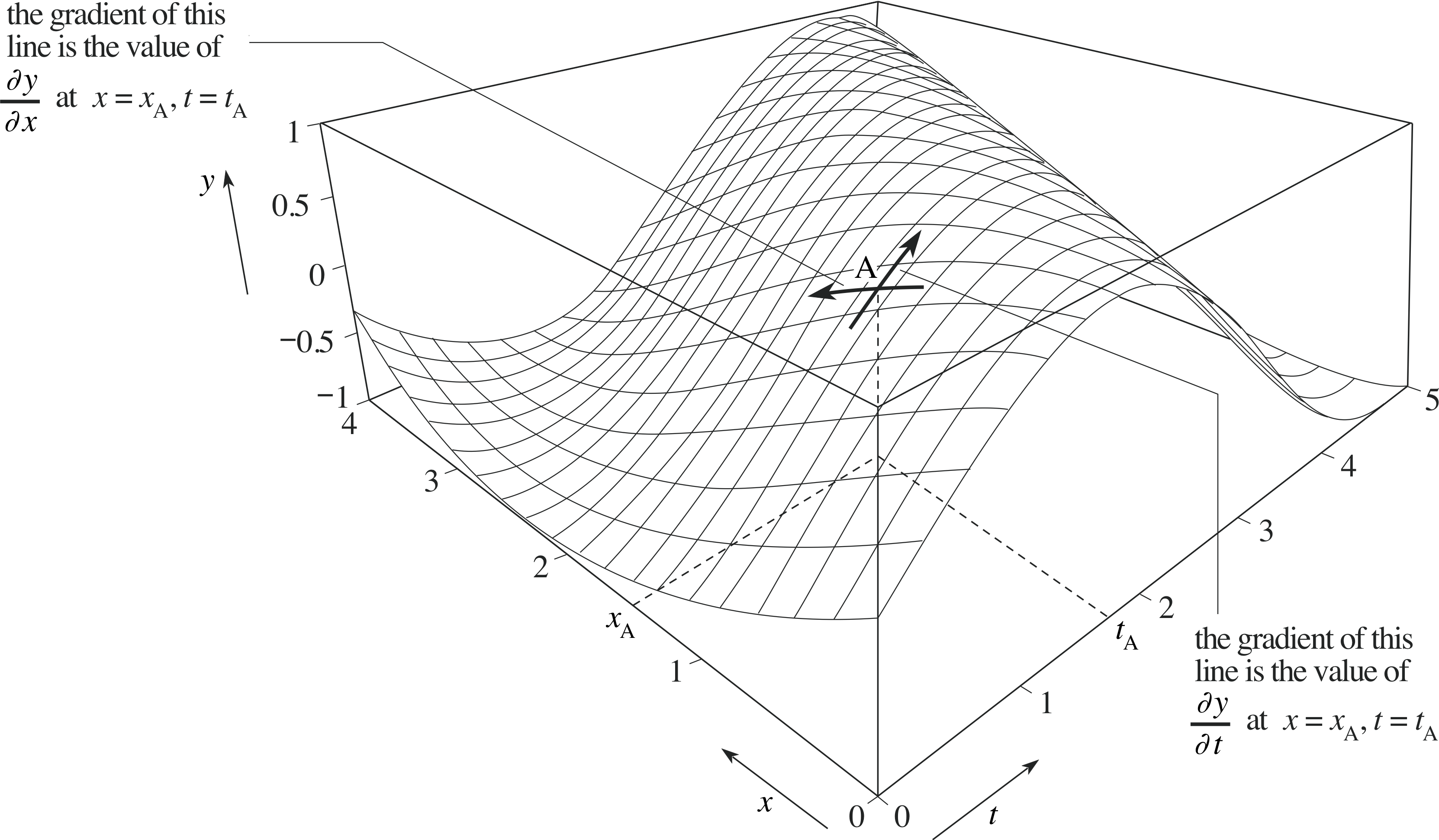
Figure 13 The graphical interpretation of the partial derivatives with respect to x and t of a function y = F (x, t) at a given point.
✦ Given that F (x, t) = (a sin kx + b cos ωt), find $\dfrac{\partial F}{\partial x}$ and $\dfrac{\partial F}{\partial t}$ and evaluate them at x = 0, t = 0.
✧ Treating t as a constant and using the chain rule
$\dfrac{\partial F}{\partial x} = 3(a\sin kx + b\cos \omega t)^2(ak\cos kx)$
Treating x as a constant and using the chain rule
$\dfrac{\partial F}{\partial t} = 3(a\sin kx + b\cos \omega t)^2(-b\omega\sin\omega t)$
At x = 0, t = 0 we therefore have
$\dfrac{\partial F}{\partial x}(0,0) = 3b^2ak\quad\text{and}\quad\dfrac{\partial F}{\partial t}(0,0) = 0$
Question T2
Given that y (x, t) = Asin[kx − ωt] find $\dfrac{\partial y}{\partial x}$ and $\dfrac{\partial y}{\partial t}$.
What is the physical significance of $\dfrac{\partial y}{\partial x}$ and $\dfrac{\partial y}{\partial t}$ if y (x, t) represents the wave of hammers moving inside the piano in the Tom and Jerry cartoon?
Answer T2
$\dfrac{\partial y}{\partial x} = Ak\cos[kx-\omega t] \quad\text{and}\quad\dfrac{\partial y}{\partial t} = -A\omega\cos[kx-\omega t$]
For a fixed value of x the graph of y = A sin[kx − ωt ] represents the wave form, i.e. the graph shows the displacement y of a particular hammer as t varies; so the partial derivative $\dfrac{\partial y}{\partial t}$ represents the y component of the velocity of a particular hammer (at fixed position x) at time t.
For a fixed value of t the graph of y = A sin[kx − ωt ] represents the wave profile, in other words the graph represents the position of all the hammers at this instant of time. The partial derivative $\dfrac{\partial y}{\partial x}$ represents the gradient of the wave profile (at the fixed instant of time) at position x.
Notice particularly that ∂ is used rather than d in the partial derivative $\left(\dfrac{\partial f}{\partial x}\right)_t$, and the t subscript can be used to
emphasize that t is to be held constant. Similarly the x subscript in $\left(\dfrac{\partial f}{\partial t}\right)_x$ can be used to emphasize that x is held constant. Usually we shall write the partial derivatives as $\dfrac{\partial f}{\partial x}$ and $\dfrac{\partial f}{\partial t}$, and drop the suffices. i
Finding partial derivatives
When dealing with partial derivatives we are by no means restricted to functions of the variables x and t. We might, for example, choose to use x and y as the independent variables, and write
z = f (x,y)
No matter what symbols we use to represent the variables, the process of finding partial derivatives involves similar techniques to finding ordinary derivatives of functions of one variable, the only difference being that we have to remember to treat one variable as a constant. An example should help to clarify this.
Example 1
If f (x, y) = x2 − y2, find $\left(\dfrac{\partial f}{\partial x}\right)_y$ and $\left(\dfrac{\partial f}{\partial y}\right)_x$.
Solution
$\left(\dfrac{\partial f}{\partial x}\right)_y = \dfrac{\partial (x^2-y^2)}{\partial x} = \dfrac{\partial (x^2)}{\partial x} - \dfrac{\partial (y^2)}{\partial x} = \dfrac{\partial (x^2)}{\partial x} = 2x$
and$\left(\dfrac{\partial f}{\partial y}\right)_x = \dfrac{\partial (x^2-y^2)}{\partial y} = \dfrac{\partial (x^2)}{\partial y} - \dfrac{\partial (y^2)}{\partial y} = -\dfrac{\partial (y^2)}{\partial y} = -2y$
There are two points to note in this example.
First, when we differentiate a function of y alone with respect to x we get zero, because y is treated as a constant. In this particular case we have $\dfrac{\partial (y^2)}{\partial x} = 0$, and similarly $\dfrac{\partial (x^2)}{\partial y} = 0$.
Second, when differentiating a function of x alone with respect to x, the partial derivative and the ordinary derivative are identical, and for this reason we can replace ∂ by d, so that, for example, $\dfrac{\partial (x^2)}{\partial x} = \dfrac{d(x^2)}{dx} = 2x$.
Example 2
Given that f (x, y) = e2x cos(3y), find $\dfrac{\partial f}{\partial x}$ and $\dfrac{\partial f}{\partial y}$.
Solution
$\dfrac{\partial f}{\partial x} = \dfrac{d({\rm e}^{2x})}{dx}\cos(3y) = 2{\rm e}^{2x}\cos(3y)$
and$\dfrac{\partial f}{\partial y} = {\rm e}^{2x}\dfrac{d(\cos(3y))}{dy} = -3{\rm e}^{2x}\sin(3y)$
Question T3
Given that f (x, y) = x2 − xy + 2y2, find $\dfrac{\partial f}{\partial x}$ and $\dfrac{\partial f}{\partial y}$.
Answer T3
$\dfrac{\partial f}{\partial x} = \dfrac{\partial}{\partial x}(x^2-xy+2y^2) = 2x - y \quad\text{and}\quad\dfrac{\partial f}{\partial y} = \dfrac{\partial}{\partial y}(x^2-xy+2y^2) = -x + 4y$
Question T4
Given that f (x, y) = x2 sin y + y2 cos x, find $\dfrac{\partial f}{\partial x}$ and $\dfrac{\partial f}{\partial y}$.
Answer T4
$\dfrac{\partial f}{\partial x} = \dfrac{\partial}{\partial x}(x^2\sin y+y^2\cos x) = 2x\sin y - y^2\sin x \quad\text{and}\quad\dfrac{\partial f}{\partial y} = \dfrac{\partial}{\partial y}(x^2\sin y+y^2\cos x) = x^2\cos y+2y\cos x$
It should be clear from these examples and questions that most of the rules of ordinary differentiation are directly applicable to partial differentiation. However, the extension of the chain rule is a little more complicated. Before using it in the context of partial differentiation let us briefly return to its application in the ordinary differentiation of a function of one variable.
✦ Given that f (x) = sin(3x2), find $\dfrac{df(x)}{dx}$.
✧ Let u = 3x2, then
$\dfrac{df(x)}{dx} = \underbrace{\dfrac{d(\sin(u))}{du}\dfrac{du}{dx}}_{\color{purple}{\large\text{Using the chain rule}}} = \cos (u)\times 6x = \underbrace{6x}_{\color{purple}{\large{du/dx}}}\cos(\underbrace{3x^2}_{\color{purple}{\large u}})$
✦ Given that ϕ (y) = sin(c2y4), where c is constant, find $\dfrac{d\varphi(y)}{dy}$.
✧ Let u = c2y4, then:
$\dfrac{d\phi(y)}{dy} = \underbrace{\dfrac{d(\sin(u))}{du}\dfrac{du}{dy}}_{\color{purple}{\large\text{Using the chain rule}}} = \cos(u)\times (4c^2y^3) = \underbrace{(4c^2y^3)}_{\color{purple}{\large{du/dx}}}\cos(\underbrace{c^2y^4}_{\color{purple}{\large u}})$
Now let us apply the same approach to a function of two variables. Naturally, we shall have to modify the chain rule somewhat to apply it in this case.
Example 3
Given that f (x, y) = sin(x2y4), find $\dfrac{\partial f}{\partial x}$ and $\dfrac{\partial f}{\partial y}$.
Solution
In this case, if we write f (x, y) = sin(u), then u = x2y4 is a function of two variables and the chain rule takes the form i
$\dfrac{\partial f}{\partial x} = \underbrace{\dfrac{d(\sin(u))}{du}\dfrac{\partial u}{\partial x}}_{\color{purple}{\large\text{Using the chain rule}}} = \cos(u)\times 2xy^4 = \underbrace{2xy^4}_{\color{purple}{\large\partial u/\partial x}}\cos(\underbrace{x^2y^4}_{\color{purple}{\large u}})$
and$\dfrac{\partial f}{\partial y} = \underbrace{\dfrac{d(\sin(u))}{du}\dfrac{\partial u}{\partial y}}_{\color{purple}{\large\text{Using the chain rule}}} = \cos(u)\times 4x^2y^3 = \underbrace{4x^2y^3}_{\color{purple}{\large\partial u/\partial y}}\cos(\underbrace{x^2y^4}_{\color{purple}{\large u}})$
In the above example, note that we use d when differentiating a function of one variable with respect to that variable, and we use ∂ when differentiating a function of several variables. Apart from that the chain rule is essentially unchanged.
Question T5
Given that f (x, t) = cosh(Ax2t3) i, where A is constant, find $\dfrac{\partial f}{\partial x}$ and $\dfrac{\partial f}{\partial y}$.
Answer T5
Setting u = Ax2t3 we have
$\dfrac{\partial f}{\partial x} = \dfrac{d\cosh(u)}{du}\dfrac{\partial u}{\partial x} = \sinh(u)\times 2Axt^3 = 2Axt^3\sinh(Ax^2t^3)$
and$\dfrac{\partial f}{\partial t} = \dfrac{d\cosh(u)}{du}\dfrac{\partial u}{\partial t} = \sinh(u)\times 3Ax^2t^2 = 3Ax^2t^2\sinh(Ax^2t^3)$
Question T6
Given that $f(x,\,y) = \loge\left(\dfrac xy\right)$, find $x\dfrac{\partial f}{\partial x}$ and $y\dfrac{\partial f}{\partial y}$.
Answer T6
First we notice that $f(x,\,y) = \loge\left(\dfrac xy\right) = \loge(x) - \loge(y)$ (since this makes the calculation a little easier), then
$\dfrac{\partial f}{\partial x} = \dfrac{\partial}{\partial x}[\loge(x)-\loge(y)] = \dfrac 1x \quad\text{and}\quad\dfrac{\partial f}{\partial y} = \dfrac{\partial}{\partial y}[\loge(x)-\loge(y)] = -\dfrac 1y$
Therefore$x\dfrac{\partial f}{\partial x}$ and $y\dfrac{\partial f}{\partial y} = 0$.
Formal definitions
The ordinary derivative df/dx of a function of a single variable f (x) is formally defined by the following limit, provided that the limit exists:
$\displaystyle \dfrac{df}{dx} = \lim_{\Delta x\rightarrow 0}{\left(\dfrac{f(x+\Delta x)-f(x)}{\Delta x}\right)}$
In a similar way, the partial derivatives of a function of two variables f (x, y) may be defined by i
$\displaystyle \left(\dfrac{\partial f}{\partial x}\right)_y = \lim_{\Delta x\rightarrow 0}{\left(\dfrac{f(x+\Delta x,\,y)-f(x,\,y)}{\Delta x}\right)}$
$\displaystyle \left(\dfrac{\partial f}{\partial y}\right)_x = \lim_{\Delta y\rightarrow 0}{\left(\dfrac{f(x,\,y+\Delta y)-f(x,\,y)}{\Delta y}\right)}$
These definitions are mainly of interest to mathematicians, but you should be able to recognize them since they can easily arise in a physical context.
2.6 Higher partial derivatives
If we are told that f (x, y) = e2x cos(3y) then we may easily find the partial derivatives
$\dfrac{\partial f}{\partial x} = 2{\rm e}^{2x}\cos(3y)\quad\text{and}\quad\dfrac{\partial f}{\partial y} = -3{\rm e}^{2x}\sin(3y)$
Now these partial derivatives are themselves functions of the two variables x and y, and so can be differentiated partially with respect to x or y.
It is generally the case that a partial derivative of a function of two variables is also a function of these variables, and if we choose we can differentiate a second time. i For example:
Iff (x, y) = e2xcos(3y)
then $\dfrac{\partial f}{\partial x} = 2{\rm e}^{2x}\cos(3y)\quad\text{and}\quad\dfrac{\partial f}{\partial y}= -3{\rm e}^{2x}\sin(3y)$
so that $\dfrac{\partial}{\partial x}\left(\dfrac{\partial f}{\partial x}\right) = \dfrac{\partial}{\partial x}\left(2{\rm e}^{2x}\cos(3y)\right) = 4{\rm e}^{2x}\cos(3y)$
while $\dfrac{\partial}{\partial y}\left(\dfrac{\partial f}{\partial y}\right) = \dfrac{\partial}{\partial y}\left(-3{\rm e}^{2x}\sin(3y)\right) = -9{\rm e}^{2x}\cos(3y)$
It is common practice to abbreviate these second partial derivatives as follows:
$\dfrac{\partial }{\partial x}\left(\dfrac{\partial f}{\partial x}\right) = \dfrac{\partial^2f}{\partial x^2}$(26)
and$\dfrac{\partial }{\partial y}\left(\dfrac{\partial f}{\partial y}\right) = \dfrac{\partial^2f}{\partial y^2}$(27)
These results are straightforward extensions of what happens with a function of one variable; here we simply differentiate with respect to x (or y) while keeping y (or x) constant. However, there are two extra possibilities which cannot occur with a function of a single variable.
Firstly, having found (in our earlier example)
$\dfrac{\partial f}{\partial x} = \underbrace{\left(\dfrac{\partial f(x,\,y)}{\partial x}\right)_{y\color{purple}{\text{ = constant}}}}_{\color{purple}{\large\substack{\text{Writing it in full}\\\text{remind you of what}\\\text{it really means}}}} = 2{\rm e}^{2x}\cos(3y)$
we could then differentiate the result with respect to y while keeping x constant. Doing this we obtain
$\dfrac{\partial }{\partial y}\left(\dfrac{\partial f}{\partial x}\right) = \dfrac{\partial}{\partial y}\left[2{\rm e}^{2x}\cos(3y)\right] = -6{\rm e}^{2x}\sin(3y)$(28)
Notice that first we keep y constant and differentiate with respect to x and then we keep x constant and differentiate with respect to y. (Notice also that we don’t use x and y subscripts to indicate which variable is being held constant since doing so would make the notation unnecessarily complicated.) We normally abbreviate these second derivatives as follows:
$\dfrac{\partial }{\partial y}\left(\dfrac{\partial f}{\partial x}\right) = \dfrac{\partial^2f}{\partial y\,\partial x}$(29)
Secondly however, we could differentiate in reverse order, so that in place of $\dfrac{\partial^2f}{\partial y\,\partial x}$ we obtain
$\dfrac{\partial }{\partial y}\left(\dfrac{\partial f}{\partial x}\right) = \dfrac{\partial}{\partial y}\left[2{\rm e}^{2x}\cos(3y)\right] = -6{\rm e}^{2x}\sin(3y)$(30)
It is no coincidence that Equations 28 and 30 give the same result, and in fact, for all the functions that you are likely to meet, it is generally true that
$\dfrac{\partial^2f}{\partial x\,\partial y} = \dfrac{\partial^2f}{\partial y\,\partial x}$(31)
The derivatives defined in Equations 29 and 31 are called mixed partial derivatives.
Example 4
If V (x, y) is defined by V (x, y) = arctan(y/x) i find $\dfrac{\partial^2V}{\partial x^2}$ and $\dfrac{\partial^2V}{\partial y^2}$.
Hence verify that V (x, y) satisfies $\dfrac{\partial^2V}{\partial x^2} + \dfrac{\partial^2V}{\partial y^2} = 0$(32)
(An equation (such as Equation 32) which involves partial derivatives is known as a partial differential equation. Equation 32 is known as Laplace’s equation (in two dimensions) and is crucial to the study of many areas of theoretical physics, including electrostatics and hydrodynamics.
Solution
Using the standard derivative (derived elsewhere in FLAP) $\dfrac{d}{du}\arctan(u) = \dfrac{1}{1+u^2}$ we obtain
$\dfrac{\partial V}{\partial x} = \dfrac{\partial}{\partial x}\left[\arctan\left(\dfrac yx\right)\right] = \dfrac{1}{1+\left(\dfrac yx\right)^2}\dfrac{\partial}{\partial x}\left(\dfrac yx\right)$ from the chain rule
$\phantom{\dfrac{\partial V}{\partial x}}= \dfrac{1}{1+\left(\dfrac yx\right)^2}\times\left(-\dfrac{y}{x^2}\right) = -\dfrac{y}{x^2+y^2}$(33)
so$\dfrac{\partial^2V}{\partial x^2} = \dfrac{2xy}{(x^2+y^2)^2}$
$\dfrac{\partial V}{\partial y} = \dfrac 1x \times \dfrac{1}{1+\left(\dfrac yx\right)^2} = \dfrac{x}{x^2+y^2}$
so$\dfrac{\partial^2V}{\partial y^2} = -\dfrac{2xy}{(x^2+y^2)^2}$
It follows that $\dfrac{\partial^2V}{\partial x^2} + \dfrac{\partial^2V}{\partial y^2} = \dfrac{x}{x^2+y^2} - \dfrac{x}{x^2+y^2}= 0$
Question T7
Given that $V(x,\,y) = \arctan\left(\dfrac yx\right)$, verify that $\dfrac{\partial^2V}{\partial y\,\partial x} = \dfrac{\partial^2V}{\partial x\,\partial y}$.
Answer T7
From Equation 33 we have $\dfrac{\partial V}{\partial x} = -\dfrac{y}{x^2+y^2} \quad\text{and so}\quad\dfrac{\partial^2V}{\partial y\partial x} = -\dfrac{1}{x^2+y^2} + \dfrac{y\times 2y}{(x^2+y^2)^2} = \dfrac{y^2-x^2}{(x^2+y^2)^2}$
From Equation 34 we have $\dfrac{\partial V}{\partial y} = \dfrac{x}{x^2+y^2} \quad\text{and so}\quad\dfrac{\partial^2V}{\partial x\partial y} = \dfrac{1}{x^2+y^2} - \dfrac{x\times 2x}{(x^2+y^2)^2} = \dfrac{y^2-x^2}{(x^2+y^2)^2}$
These two results show that $\dfrac{\partial^2V}{\partial y\partial x} = \dfrac{\partial^2V}{\partial x\partial y}$
Question T8
If V (r, θ) = (αr n + βr−n) cos(nθ) where α, β and n are constants, find $\dfrac{\partial V}{\partial r}, \dfrac{\partial^2V}{\partial r^2}\text{ and }\dfrac{\partial^2V}{\partial\theta^2}$.
Hence show that
$\dfrac{\partial^2V}{\partial r^2} + \dfrac 1r \dfrac{\partial V}{\partial r}+\dfrac{1}{r^2}\dfrac{\partial^2V}{\partial\theta^2} = 0$(35)
Answer T8
$\dfrac{\partial V}{\partial r} = \left[\alpha nr^{n-1}-\beta nr^{-(n+1)}\right]\cos(n\theta)$
$\dfrac{\partial^2V}{\partial r^2} = \left[\alpha n(n-1)r^{n-2}+\beta n(n+1)r^{-(n+2)}\right]\cos(n\theta)$
$\dfrac{\partial V}{\partial\theta} = -n\left[\alpha r^n + \beta r^{-n}]\sin(n\theta)\right]$ and
$\dfrac{\partial^2V}{\partial\theta^2} = -n^2\left[\alpha r^n + \beta r^{-n}]\cos(n\theta)\right]$
and therefore $\dfrac{\partial^2V}{\partial r^2} + \dfrac 1r \dfrac{\partial V}{\partial r} + \dfrac{1}{r^2}\dfrac{\partial^2V}{\partial\theta^2}$
$= \left[\alpha n(n-1)r^{n-2}+\beta n(n+1)r^{-(n+2)}\right]\cos(n\theta) + \dfrac 1r\left[\alpha nr^{n-1}-\beta nr^{-(n+1)}\right]\cos(n\theta) - \dfrac{n^2}{r^2}\left[\alpha r^n + \beta r^{-n}\right]\cos(n\theta)$
$= \left[n(n-1)+n-n^2\right]\alpha r^{n-2}\cos(n\theta) + \left[\alpha n{n+1}-n-n^2\right]\beta r^{-(n+2)}\cos(n\theta) = 0$
Question T9
The pressure P, temperature T and volume V of a certain gas are related by van der Waals’ equation i
$\left(P+\dfrac{a}{V^2}\right)(V-b) = RT$(36)
where a, b and R are all constant. Regarding P as a function of V and T, find the values of P, V and T (in terms of the constants a, b and R) for which the equations
$\dfrac{\partial P}{\partial V}= 0\quad\text{and}\quad\dfrac{\partial^2P}{\partial V^2}= 0$
are satisfied simultaneously.
Answer T9
Rearranging Equation 36 to give an expression for P, we get
$P = \dfrac{RT}{V-b} - \dfrac{a}{V^2}$(i)
so that$\dfrac{\partial P}{\partial V} = \dfrac{-RT}{(V-b)^2} + \dfrac{2a}{V^3}$
and$\dfrac{\partial^2P}{\partial V^2} = \dfrac{2RT}{(V-b)^3} - \dfrac{6a}{V^4}$
Setting $\dfrac{\partial P}{\partial V} = 0$ gives
$\dfrac{RT}{(V-b)^2} = \dfrac{2a}{V^3}$(ii)
and setting $\dfrac{\partial^2P}{\partial V^2} = 0$ gives
$\dfrac{2RT}{(V-b)^3} = \dfrac{6a}{V^4}$(iii)
Dividing Equation (ii) by Equation (iii) we obtain
$V - b = \dfrac 23 V$(iv)
and therefore V = 3b
Substituting this result into Equation (ii) gives
$\dfrac{RT}{(3b-b)^2} = \dfrac{2a}{27b^3}$
and therefore $T = \dfrac{8a}{27bR}$
Putting these expressions for V (V = 3b) and T in Equation (i), we obtain
$P = \dfrac{R}{(3b - b)}\times \dfrac{8a}{27bR} - \dfrac{a}{9b^2} = \dfrac{a}{27b^2}$
2.7 The wave equation
A general wave
In Subsection 2.4 we showed that a general one–dimensional wave that travels with unchanging shape at constant speed v has the form y = f (x ± vt). We now set out to find the equation for which this is a solution. i For this restricted class of functions of two variables it is possible to simplify the process of finding the partial derivatives. If we put u = x ± vt, then we can find the partial derivatives of f with respect to x in terms of the derivative with respect to u. i
✦ Given that f (x, t) = sin(x + vt), find $\dfrac{\partial f}{\partial x}$, then put u = x + vt and calculate$\dfrac{\partial f}{\partial u}$.
Hence show that $\dfrac{\partial f}{\partial x} = \dfrac{\partial f}{\partial u}$ in this case.
✧ $\dfrac{\partial f}{\partial x} = \cos(x+vt)$
With f (u) = sin(u) we have
$\dfrac{df}{du} = \cos(u) = \cos(x+vt)$
Hence, as required $\dfrac{\partial f}{\partial x} = \dfrac{df}{du}.$
It is no accident that $\dfrac{\partial f}{\partial x} = \dfrac{\partial f}{\partial u}$ in the previous exercise. If u = x ± vt we have $\dfrac{\partial u}{\partial x} = 1$, and we can use the chain rule to write
$\dfrac{\partial f}{\partial x} = \dfrac{\partial f}{\partial u}\underbrace{\dfrac{\partial u}{\partial x}}_{\color{purple}{\large\substack{\text{This is}\\\text{equal}\\\text{to 1}}}} = \dfrac{\partial f}{\partial u}$(37) i
✦ Given that f (x, t) = sin(x + vt), find $\dfrac{\partial f}{\partial t}$, then put u = x + vt and calculate $v\dfrac{\partial f}{\partial u}$.
Hence show that $\dfrac{\partial f}{\partial t} = v\dfrac{\partial f}{\partial u}$ in this case.
✧ $\dfrac{\partial f}{\partial t} = v\cos(x+vt)$
With f (u) = sin(u) we have
$\dfrac{df}{du} = \cos(u) = \cos(x+vt)$
and therefore
$v\dfrac{df}{du} = v\cos(x+vt)$
Hence, as required $\dfrac{\partial f}{\partial t} = v\dfrac{df}{du}.$
Once again, this result is no accident since if u = x ±vt then $\dfrac{\partial u}{\partial t} = \pm v$, and the chain rule gives
$\dfrac{\partial f}{\partial t} = \dfrac{\partial f}{\partial u}\underbrace{\dfrac{\partial u}{\partial t}}_{\color{purple}{\large\substack{\text{This is}\\[1pt]\text{equal}\\[0pt]\text{to }\pm v}}} = \pm v \dfrac{\partial f}{\partial u}$(38)
We can now use a similar process to find the second–order partial derivatives. Since df can also be regarded as du
a function of x and t, we can differentiate once again with respect to x to obtain
$\dfrac{\partial^2f}{\partial x^2} = \underbrace{\dfrac{\partial}{\partial x}\left(\dfrac{\partial f}{\partial x}\right)}_{\color{purple}{\large\substack{\text{This is just}\\[0pt]\text{the definition}\\[1pt]\text{of the second}\\[1pt]\text{derivative}}}} = \dfrac{\partial}{\partial x}\underbrace{\left(\dfrac{\partial f}{\partial u}\right)}_{\color{purple}{\large\substack{\text{From}\\[2pt]\text{Eqn 37}}}} = \underbrace{\dfrac{d}{du}\left(\dfrac{df}{du}\right)}_{\color{purple}{\large\substack{\text{This comes from}\\[2pt]\text{Eqn 37 with } df/du\\[1pt]\text{in place of }f}}} = \dfrac{d^2f}{du^2}$(39)
Similar operations i can be performed with respect to t, so that
$\dfrac{\partial^2f}{\partial x^2} = \dfrac{\partial}{\partial t}\left(\pm v\dfrac{\partial f}{\partial u}\right) = \pm v\dfrac{d^2f}{du^2}\dfrac{\partial u}{\partial t} = \left(\pm v\right)^2\dfrac{\partial^2f}{\partial u^2} = v^2\dfrac{d^2f}{du^2}$(40)
We can now eliminate $\dfrac{d^2f}{du^2}$ from Equations 39 and 40 to obtain
$\dfrac{\partial^2f}{\partial x^2} - \dfrac{1}{v^2}\dfrac{\partial^2f}{\partial t^2} = 0$(41)
This is a second–order partial differential equation with the required solution, and is known as the (one-dimensional) wave equation. Many interesting physical quantities can be shown to satisfy this equation, and very often we would like to find its solution subject to various boundary conditions. From our previous discussion we know that any function of the form y (x, t) = f (x ± vt) is a solution of Equation 41, but there are two points to appreciate here. First, this may not be the most general solution; and second, we usually need to find some particular solution in order to solve a given problem.
So there are two important questions to consider: what is the most general solution of Equation 41, and how can one select a solution that solves a given problem from this vast array of possible solutions? We shall not be able fully to answer these questions in this module, but we shall show that certain specific functions are indeed solutions of Equation 41. i We shall also discuss some general features of solutions to the wave equation.
Question T10
Show that if two functions f1 and f2 are solutions of the wave equation
$\dfrac{\partial^2f}{\partial x^2} - \dfrac{1}{v^2}\dfrac{\partial^2f}{\partial t^2} = 0$
then any function of the form αf1 + βf2, where α and β are arbitrary constants, is also a solution.
Answer T10
Suppose f1(x, t) and f2(x, t) satisfy the wave equation, that is
$\dfrac{\partial^2f_1}{\partial x^2} - \dfrac{1}{v^2}\dfrac{\partial^2f_1}{\partial t^2} = 0$(i)
and$\dfrac{\partial^2f_2}{\partial x^2} - \dfrac{1}{v^2}\dfrac{\partial^2f_2}{\partial t^2} = 0$(ii)
Taking the sum of α × Equation (i) and β × Equation (ii) gives
$\alpha\dfrac{\partial^2f_1}{\partial x^2} + \beta\dfrac{\partial^2f_2}{\partial x^2} - \alpha \dfrac{1}{v^2}\dfrac{\partial^2f_1}{\partial t^2} - \beta \dfrac{1}{v^2}\dfrac{\partial^2f_2}{\partial t^2} = 0$
However in general $\dfrac{\partial^2}{\partial x^2}(\alpha f_1 + \beta f_2) = \alpha\dfrac{\partial^2f_1}{\partial x^2} + \beta\dfrac{\partial^2f_2}{\partial x^2}$
(with a similar result for differentiating with respect to t) and therefore
$\dfrac{\partial^2}{\partial x^2}(\alpha f_1 + \beta f_2) - \dfrac{1}{v^2}\dfrac{\partial^2}{\partial t^2}(\alpha f_1 + \beta f_2) = 0$
This shows that αf1+ βf2 is also a solution of the wave equation.
Comment This result is sometimes known as the superposition principle since it implies that we can obtain new solutions by superposing (that is, adding) the known ones. Mathematically, this is true because the wave equation is linear in the function f (x, y).
Partial differential equations are very common throughout physics and there is a large literature devoted to techniques which in some circumstances lead to explicit solutions. i No matter what method is used to find a solution, it can always be verified by substituting back into the differential equation. We shall be concerned with showing that we really do have a solution to the wave equation, rather than with general techniques for finding solutions.
✦ Verify that y (x, t) = A sin(ωt − kx + ϕ) is a solution of a wave equation of the form
$\dfrac{\partial^2f}{\partial x^2} - \dfrac{1}{v^2}\dfrac{\partial^2f}{\partial t^2} = 0$(Eqn 41)
provided we identify f with y, and provided v2 = ω2/k2.
✧ $\dfrac{\partial y}{\partial x} = -kA\cos(\omega t - kx + \phi) \quad\text{and}\quad\dfrac{\partial y}{\partial t} = \omega A\cos(\omega t - kx + \phi)$
$\dfrac{\partial}{\partial x}\left(\dfrac{\partial y}{\partial x}\right) = \dfrac{\partial}{\partial x}\left(-kA\cos(\omega t - kx + \phi)\right) = -k^2A\sin(\omega t - kx + \phi)$
$\dfrac{\partial}{\partial t}\left(\dfrac{\partial y}{\partial t}\right) = \dfrac{\partial}{\partial x}\left(\omega A\cos(\omega t - kx + \phi)\right) = -\omega^2A\sin(\omega t - kx + \phi)$
and therefore $\dfrac{1}{k^2}\dfrac{\partial^2y}{\partial x^2} = \dfrac{1}{\omega^2}\dfrac{\partial^2y}{\partial t^2}$
which gives the required result.
2.8 Deriving the wave equation
We have shown that the function y (x, t) = Asin(ωt − kx + ϕ) is a solution of the wave equation (Equation 41),
$\dfrac{\partial^2f}{\partial x^2} - \dfrac{1}{v^2}\dfrac{\partial^2f}{\partial t^2} = 0$(Eqn 41)
but why should there be waves on the surface of a lake, on a string or sound waves in air? How do we know that such physical systems are governed, at least approximately, by the wave equation?
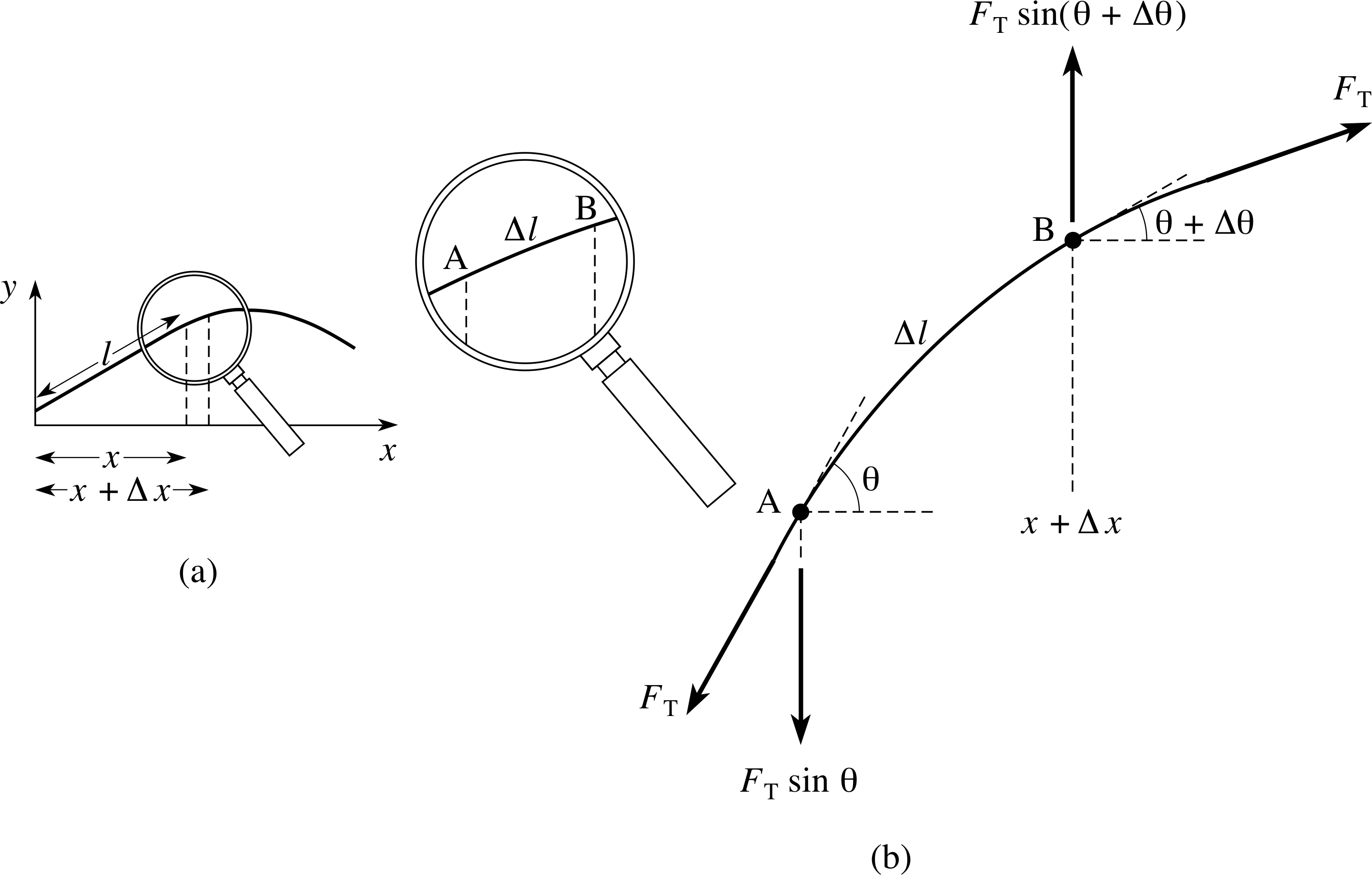
Figure 14 (a) A vibrating string, and (b) an enlargement of the segment AB.
As an example of how waves occur in physical systems, we now derive the wave equation for a stretched string. Other physical systems, such as sound waves in air, can be analysed in a similar way.
We start by considering a segment AB of the string which is of length ∆l, as shown in Figure 14. The string is assumed to be stretched tightly along the horizontal x–direction, and then set in motion in the y -direction perpendicular to its length. (We ignore the effects of gravity in the following discussion.)
The angle θ is the angle between the tangent to the curve and the x–direction, and it will be small if the oscillations in the string are small. i
The following quantities are needed in our derivation:
x = position of one end of the segment as measured from a fixed point along the line of the string when at rest;
t = time at which the segment is in the position shown;
y (x, t) = displacement from the rest position of the segment ΑΒ;
FT = the magnitude of the force acting on the ends of the string due to tension in the string (assumed to be constant);
μ = the mass per unit length of the string (the linear mass density);
θ = the angle associated with the point at the ‘lower’ end of the segment;
θ + ∆θ = the angle associated with the point at the ‘upper’ end of the segment.
The mass of the segment is μ ∆l which is approximately μ∆x if θ is small (the size of θ has been exaggerated in the figure). Resolving the forces acting on the segment, as in Figure 14b, shows that there is a net transverse force which causes the segment to accelerate in the y–direction.
In other words, we treat x as a constant and differentiate y twice partially with respect to t to obtain the acceleration $\dfrac{\partial^2y}{\partial t}$ of the segment.
Newton’s second law enables us to relate the acceleration to the force as follows
$\underbrace{\mu\Delta x}_{\color{purple}{\large\substack{\text{mass}\\[2pt]\text{of AB}}}} \underbrace{\dfrac{\partial^2y}{\partial t^2}}_{\color{purple}{\large\substack{\text{acceleration}\\[2pt]\text{of AB in}\\[2pt]\text{the }y\text{-direction}}}} = \underbrace{F_{\rm T}\sin(\theta + \Delta\theta) - F_{\rm T}\sin(\theta)}_{\color{purple}{\large\substack{y\text{-component of the}\\[2pt]\text{force acting on AB}}}}$(42)
However for small angles we have sin(θ) ≈ tan(θ) so that Equation 42 can also be written:
$\mu\Delta x \dfrac{\partial^2y}{\partial t^2} = F_{\rm T}\tan(\theta + \Delta\theta) - F_{\rm T}\tan(\theta)$(43)
Suppose now that we keep t fixed, and consider the function f (x) defined by
f (x) = y (x, t)
for constant t, the graph of which is shown in Figure 14a. The gradient of this graph at the point A is
f ′ (x) = tan θ
while the gradient of the graph at the point B is
f ′ (x + ∆x) = tan(θ + ∆θ)
This means that we can rewrite the right–hand side of Equation 43 to obtain
$\mu\Delta x \dfrac{\partial^2y}{\partial t^2} = \dfrac{F_{\rm T}f'(x + \Delta x) - F_{\rm T}f'(x)}{\Delta x}$(44)
so that$\dfrac{\mu}{F_{\rm T}}\dfrac{\partial^2y}{\partial t^2} = \dfrac{f'(x + \Delta x) - f'(x)}{\Delta x}$
If we now take the limit as ∆x tends to zero, the approximation becomes increasingly accurate, and therefore (see Question R3) i
$\dfrac{\mu}{F_{\rm T}}\dfrac{\partial^2y}{\partial t^2} = f''(x)$(45)
However, we defined f (x) to be equal to y (x, t) for constant t, so that $f''(x) = \dfrac{\partial^2y}{\partial x^2}$, and this means that Equation 45 becomes
$\dfrac{\mu}{F_{\rm T}}\dfrac{\partial^2y}{\partial t^2} = \dfrac{\partial^2y}{\partial x^2}$(46)
Now if we identify μ/FT with 1/v2 we see that Equation 46 is actually a form of the wave equation.
This shows that small amplitude waves on a stretched string propagate with a speed v given by
$v = \sqrt{\dfrac{F_{\rm T}\os}{\mu}}$(47) i
Question T11
The y–component of an electric field Ey(x, t) and the z–component of a magnetic field Bz(x, t) are related by the partial differential equations i
$\dfrac{\partial B_z}{\partial t} = -\dfrac{\partial E_y}{\partial x}$(48)
$\mu_0\varepsilon_0\dfrac{\partial E_y}{\partial t} = -\dfrac{\partial B_z}{\partial x}$(49)
where μ0 and ε0 are constants. Show that Ey and Bz both satisfy wave equations, and in each case find the speed of the wave. [Hint: Differentiate one equation with respect to t and the other respect to x.]
Study comment It turns out that any pair of physical quantities, f (x, t) and g (x, t), which satisfy the pair of differential equations
$\dfrac{\partial f}{\partial t} = \alpha\dfrac{\partial g}{\partial x}\quad\text{and}\quad\dfrac{\partial g}{\partial t} = \beta\dfrac{\partial f}{\partial x}$
where α and β are constants, lead to wave equations for f and g.
Answer T11
Differentiating Equation 48 with respect to t
$\dfrac{\partial B_z}{\partial t} = -\dfrac{\partial E_y}{\partial x}$(Eqn 48)
and Equation 49 with respect to x
$\mu_0\varepsilon_0\dfrac{\partial E_y}{\partial t} = -\dfrac{\partial B_z}{\partial x}$(Eqn 49)
we get$\dfrac{\partial^2B_z}{\partial t^2} = -\dfrac{\partial^2E_y}{\partial t\partial x}$(i)
and$\mu_0\varepsilon_0\dfrac{\partial^2E_y}{\partial x\partial t} = -\dfrac{\partial B_z}{\partial x^2}$(ii)
Now $\dfrac{\partial^2E_y}{\partial t\partial x} = \dfrac{\partial^2E_y}{\partial x\partial t}$, so Equations (i) and (ii) give
$\mu_0\varepsilon_0\dfrac{\partial^2B_z}{\partial t^2} = \dfrac{\partial^2B_z}{\partial x^2}$
so that$\dfrac{\partial^2B_z}{\partial x^2} - \dfrac{1}{v^2}\dfrac{\partial^2B_z}{\partial t^2} = 0$
where$v = \dfrac{1}{\sqrt{\mu_0\varepsilon_0\os}}$
In a similar way, if we differentiate Equation 48 with respect to x and Equation 49 with respect to t we get
we get$\dfrac{\partial^2B_z}{\partial x\partial t} = -\dfrac{\partial^2E_y}{\partial x^2}$(iii)
and$\mu_0\varepsilon_0\dfrac{\partial^2E_y}{\partial t^2} = -\dfrac{\partial B_z}{\partial t\partial x}$(iv)
Now $\dfrac{\partial^2B_z}{\partial t\partial x} = \dfrac{\partial^2B_z}{\partial x\partial t}$, so Equations (iii) and (iv) give
$\mu_0\varepsilon_0\dfrac{\partial^2E_y}{\partial t^2} = \dfrac{\partial^2E_y}{\partial x^2}$
so that$\dfrac{\partial^2E_y}{\partial x^2} - \dfrac{1}{v^2}\dfrac{\partial^2E_y}{\partial t^2} = 0$
where$v = \dfrac{1}{\sqrt{\mu_0\varepsilon_0\os}}$
Comment Wave equations can be derived from any pair of equations with the same structure as Equations 48 and 49.
The general technique is to first differentiate one equation with respect to the time variable and the other equation with respect to the position variable, and then to eliminate the mixed derivative terms.
Energy flow for a wave on a string
If a wave propagates along a string there is an instantaneous flow of energy past a fixed point on the string. i As a pulse moves past a particular point there is clearly energy present at that point (since the string is moving) but, once the wave has moved on, the energy returns to zero (since the string is locally at rest). We can see this mathematically by observing that the instantaneous rate of flow of energy past a point x on the string, i.e. the power P, is equal to the product of the upward force on the point multiplied by the transverse component of the string’s velocity $\dfrac{\partial y}{\partial t}$. (The component of velocity of the segment along the string is assumed to be negligibly small.)
✦ Would it be more sensible to write ‘speed’ rather than ‘the transverse component of velocity’?
✧ No! Whereas speed is a magnitude and must be positive, $\dfrac{\partial y}{\partial t}$ can be positive or negative depending on the direction of motion.
From our earlier discussion we know that the component of force in the y–direction at the point A is
$-F_{\rm T}\sin\theta \approx -F_{\rm T}\tan\theta = -F_{\rm T}\dfrac{\partial y}{\partial x}$(50)
and therefore the power is given by
$P = -F_{\rm T}\dfrac{\partial y}{\partial x}\dfrac{\partial y}{ \partial t}$(51)
If we consider a wave moving from left to right, then y (x, t) = f (x − vt) and, putting u = x − vt, we obtain (from Equations 37 and 38)
$\dfrac{\partial f}{\partial x} = \dfrac{\partial f}{\partial u}\underbrace{\dfrac{\partial u}{\partial x}}_{\color{purple}{\large\substack{\text{This is}\\\text{equal}\\\text{to 1}}}} = \dfrac{\partial f}{\partial u}$(Eqn 37)
$\dfrac{\partial f}{\partial t} = \dfrac{\partial f}{\partial u}\underbrace{\dfrac{\partial u}{\partial t}}_{\color{purple}{\large\substack{\text{This is}\\[1pt]\text{equal}\\[0pt]\text{to }\pm v}}} = \pm v \dfrac{\partial f}{\partial u}$(Eqn 38)
$\dfrac{\partial y}{\partial t} = \dfrac{\partial f}{\partial u}\dfrac{\partial u}{\partial t} = -v\dfrac{\partial f}{\partial u}\quad\text{and}\quad\dfrac{\partial y}{\partial x} = \dfrac{\partial f}{\partial u}\dfrac{\partial u}{\partial x} = \dfrac{\partial f}{\partial u}$
Hence, from Equation 51, the power is given by
$P = vF_{\rm T}\left(\dfrac{df}{du}\right)^2$(52)
The sign of P shows that the energy flows from left to right for a wave that travels from left to right.
✦ Show that P is negative for a wave moving from right to left.
✧ A wave that moves from right to left has the form y (x, t) = g (x + vt) and putting w = x + vt, we obtain
$\dfrac{\partial y}{\partial t} = \dfrac{dg}{dw}\dfrac{\partial w}{\partial t} = v\dfrac{dg}{dw}\quad\text{and}\quad\dfrac{\partial y}{\partial x} = \dfrac{dg}{dw}\dfrac{\partial w}{\partial x} = \dfrac{dg}{dw}$
Equation 52,
$P = vF_{\rm T}\left(\dfrac{df}{du}\right)^2$(Eqn 52)
now gives $P = -vF_{\rm T}\left(\dfrac{dg}{dw}\right)^2$, and the fact that P is negative shows that the energy flows from right to left.
2.9 Standing waves
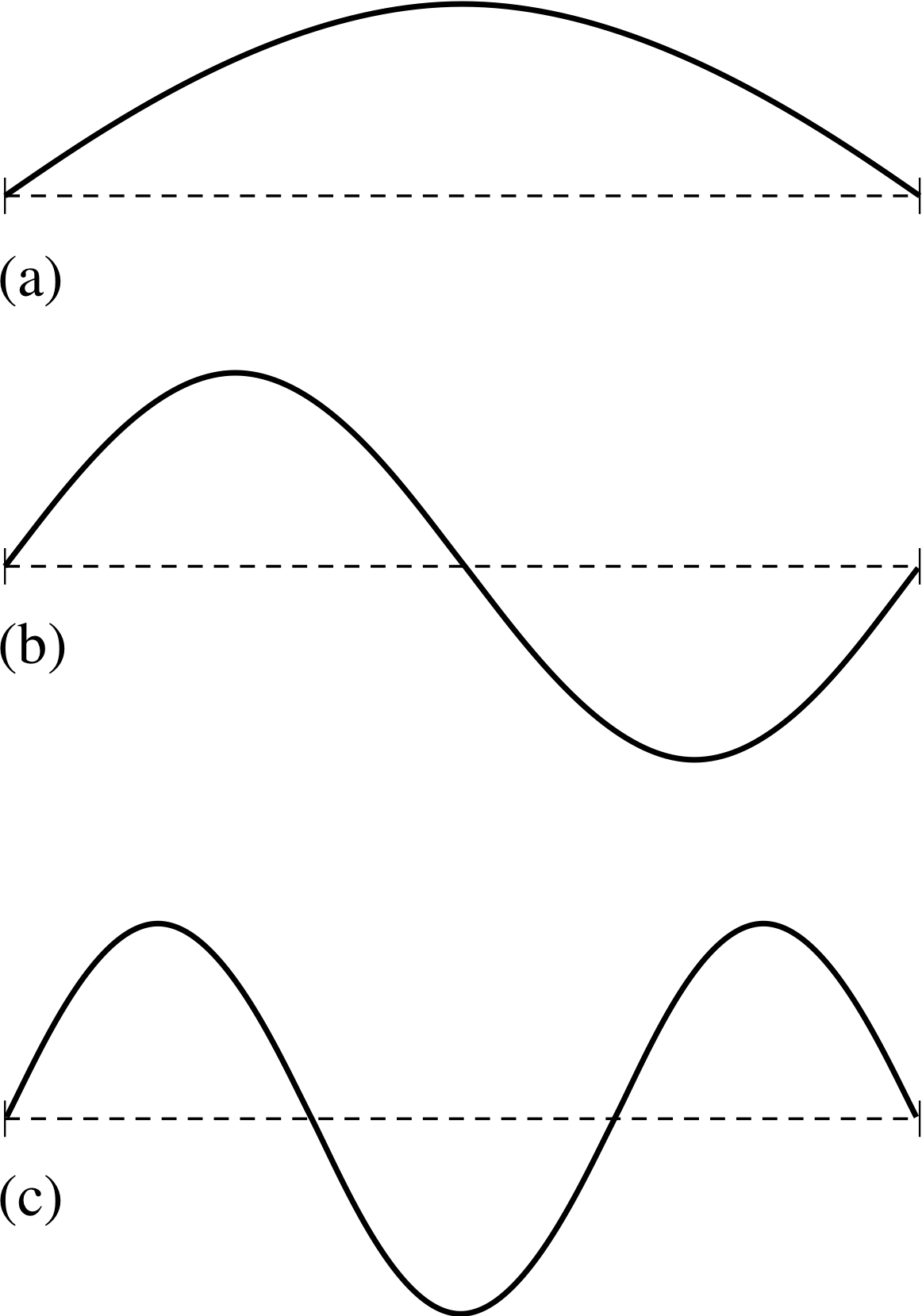
Figure 15 Standing waves for a string fixed at its ends. This is the wave profile, and the horizontal axis is distance.
So far we have visualized waves as fixed shapes which change position, and we have referred to such waves as travelling waves. However, not all waves are travelling waves. Figure 15 shows three of the ways in which a stretched string with fixed endpoints can be made to move. In each case the displacement of the string from its equilibrium position is a function of position and time, and will satisfy the wave equation. Yet in this case the ‘waves’ are not going anywhere; they do not appear to travel to the left or to the right. In fact, they are called standing waves. On a standing wave there are some positions, called nodes, at which the displacement is always zero.
As we will now demonstrate, a standing wave can be regarded as a particular combination of progressive waves which are travelling in opposite directions. i Consider the sum of two progressive waves which have the same angular frequencies and wavenumbers but are moving in opposite directions
y (x, t) = C sin(ωt − kx + ϕ1) + D sin(ωt + kx + ϕ2)(53)
and suppose we are looking for standing waves in the stretched string shown in Figure 15. Let the string be of length L. The parameters in the expression for y (x, t) are not completely arbitrary since y (x, t) must satisfy the condition that neither end of the string can move.
If x = 0 corresponds to one end of the string, then this implies that
y (0, t) = 0 for all values of t(54)
and therefore
C sin(ωt + ϕ1) + D sin(ωt + ϕ2) = 0 for all values of t
Since this equation is true for all values of t the functions Csin(ωt + ϕ1) and −Dsin(ωt + ϕ2) must be identical, and this implies that
C = −D and ϕ1 = ϕ2.
If we replace ϕ1 and ϕ2 by ϕ, and D by −C our solution (Equation 53) to the wave equation reduces to
y (x, t) = C [sin(ωt − kx + ϕ) − sin(ωt + kx + ϕ)]
This expression can be converted into a more convenient form by using the trigonometric identity
$\sin\alpha - \sin\beta = 2\sin\left(\dfrac{\alpha-\beta}{2}\right)\cos\left(\dfrac{\alpha+\beta}{2}\right)$(55)
to give: y (x, t) = −2C cos(ωt + ϕ) sin(kx)(56)
The point (0, L) corresponds to the other end of the string, which is also fixed; so y (L, t) = 0 for all values of t.
So,cos(ωt + ϕ) sin(kL) = 0(57)
Since this is also true for all values of t, we must have
sin(kL) = 0(58)
The sine function is zero only when its argument is an integer multiple of π, so it follows that
kL = nπ where n = 0, ±1, ±2, ...(59)
Equation 59 is of profound importance because it tells us that the value of k cannot be chosen arbitrarily; only certain values of k are possible if this end of the string is to remain fixed. Substituting the allowed values of k = nπ/L in Equation 56 we find all the allowed forms of sinusoidal standing waves that can exist on a string of length L with fixed end points
$y(x,\,t) = A\cos(\omega t + \varphi)\sin\left(\dfrac{n\pi x}{L}\right)$ where n = 1, 2, 3, ...(60)
Notice that in writing Equation 60 we have replaced −2C by A for convenience and we have dropped the non–positive values of n. The negative values of n do not lead to expressions for y (x, t) which are independent of the positive values since
$\sin\left(-\dfrac{n\pi x}{L}\right) = -\sin\left(\dfrac{n\pi x}{L}\right)$ i
and all these waves can be reproduced by selecting an appropriate value for the phase constant ϕ.
Also note that the ‘wave’ corresponding to n = 0 in Equation 60 is the trivial case of the string at rest and is therefore of little interest.
✦ (a) What values of n in the function
$y(x,\,t) = A\cos(\omega t + \phi)\sin\left(\dfrac{n\pi x}{L}\right)$
correspond to the three standing waves of Figure 15?
(b) What expressions for y (x, t) correspond to these standing waves in Figure 15?
✧ (a) The waves correspond to n = 1, 2 and 3 since they have 0, 1, and 2 nodes respectively.
(b) The expressions for y (x, t) are
$y(x,\,t) = A\cos(\omega t + \phi)\sin\left(\dfrac{\pi x}{L}\right)$
$y(x,\,t) = A\cos(\omega t + \phi)\sin\left(\dfrac{2\pi x}{L}\right)$ and
$y(x,\,t) = A\cos(\omega t + \phi)\sin\left(\dfrac{3\pi x}{L}\right)$
The values for ϕ in the above function are indeterminate, since the wave profile tells us nothing about time. Although each expression for y (x, t) given by a particular value of n is a solution of the wave equation
$\dfrac{\partial^2y}{\partial x^2} - \dfrac{1}{v^2}\dfrac{\partial^2y}{\partial t^2} = 0$
these waves do not appear to propagate with speed v since they are in fact standing waves. As we have just demonstrated, each of these standing waves is actually the sum of two progressive waves travelling in opposite directions with speed v. The standing waves cannot be expressed as a single function of f (x ± vt), since they are always combinations of two such functions with opposite signs within the bracket.
✦ Are the frequencies of the standing waves that we have found for the stretched string arbitrary?
✧ No! A standing wave must have k = nπ L with n = 1, 2, 3... and, since ω = 2πf and v = ω/k, the permitted frequencies are given by
$f = \dfrac{\omega}{2\pi} = \dfrac{vk}{2\pi} = \dfrac{vn}{2L}$ for n = 1, 2, 3... i
This means that we can write the standing waves as
$y(x,\,t) = A\cos\left(\dfrac{n\pi vt}{L} + \phi\right)\sin\left(\dfrac{n\pi x}{L}\right)$ where n = 1, 2, 3...(61)
Study comment Make sure you study the answer to the above question. The answer is important in its own right, but it also leads on to the important finding that:
The standing waves can be written in the form
$y(x,\,t) = A\cos\left(\dfrac{n\pi vt}{L} + \phi\right)\sin\left(\dfrac{n\pi x}{L}\right)$ where n = 1, 2, 3...(Eqn 61)
Question T12
If the standing waves on a string are described by the function y (x, t) given in Equation 61, show that the rate of energy flow past a fixed point x on the string is given by
$P =F_{\rm T}v\left(\dfrac{n\pi A}{2L}\right)^2\sin\left(\dfrac{2n\pi vt}{L} + 2\phi\right)\sin\left(\dfrac{2n\pi x}{L}\right)$
Also find the values of P at x = 0 and x = L and explain your results.
[Hints: The previous section gives an expression for P in terms of partial derivatives, and you may need to use the identity sin(2θ) = 2 sin(θ) cos(θ).]
Answer T12
Using the expression for the power P given in Equation 51,
$P = -F_{\rm T}\dfrac{\partial y}{\partial x}\dfrac{\partial y}{ \partial t}$(Eqn 51)
it is clear that we need to find $\dfrac{\partial y}{\partial x} \;\text{and}\; \dfrac{\partial y}{\partial t}$.
From Equation 61,
$y(x,\,t) = A\cos\left(\dfrac{n\pi vt}{L} + \phi\right)\sin\left(\dfrac{n\pi x}{L}\right)$ where n = 1, 2, 3...(Eqn 61)
we have
$\dfrac{dy}{dx} = \dfrac{n\pi A}{L}\cos\left(\dfrac{n\pi vt}{L} + \phi\right)\cos\left(\dfrac{n\pi x}{L}\right)$
and$\dfrac{dy}{dt} = -\dfrac{n\pi vA}{L}\sin\left(\dfrac{n\pi vt}{L} + \phi\right)\sin\left(\dfrac{n\pi x}{L}\right)$
Substituting these results into Equation 51 we obtain
$P = F_{\rm T}v\left(\dfrac{n\pi A}{L}\right)^2\cos\left(\dfrac{n\pi vt}{L} + \phi\right)\cos\left(\dfrac{n\pi x}{L}\right) \times \sin\left(\dfrac{n\pi vt}{L} + \phi\right)\sin\left(\dfrac{n\pi x}{L}\right)$
$\phantom{P }= F_{\rm T}v\left(\dfrac{n\pi A}{L}\right)^2\sin\left(\dfrac{2n\pi vt}{L} + 2\phi\right)\sin\left(\dfrac{2n\pi x}{L}\right)$
where we have used the identity sin(2θ) = 2 sin(θ) cos(θ).
We can see that P = 0 at x = 0 (since sin(0) = 0) and P = 0 at x = L since sin(2πn) = 0. Both ends of the string are
stationary and therefore we would not expect energy to flow past these points.
3 The Schrödinger equation
Study comment The Schrödinger equation is the central equation of quantum mechanics. The purpose of this section is to introduce the Schrödinger equation as another example of a partial differential equation with wave–like solutions, and to examine some of its mathematical properties – it is not designed to teach you quantum mechanics. A very brief survey of quantum mechanics is contained in Subsection 3.1, to enable you see something of the physical context in which the Schrödinger equation arises, but for a comprehensive introduction to this very important part of physics you should consult the appropriate modules in the physics strand of FLAP.
3.1 The time–dependent Schrödinger equation
In the early years of the 20th century it became increasingly apparent that classical physics – the newtonian mechanicsmechanics of Newton, the maxwells_theory_of_electromagnetismelectromagnetism of James_Clerk_MaxwellMaxwell, the thermodynamics of Clausius, and so on – was incapable of accounting for many of the phenomena involving atoms and nuclei that were being discovered at that time. Because of this the period from 1900 to 1925 saw the development of a number of poorly formulated ‘theories’ that tried to explain the new phenomena in terms of an ad hoc mix of classical ideas and radical new proposals. The need for a new theoretical framework to replace classical physics, one that would bring old and new ideas together in a more coherent way, was widely perceived, but the experimental data were so fragmentary, and the required shift in thinking so great that it was not until 1925/26 that the way forward became clear. It was during these years that a relatively small number of European physicists including Werner Heisenberg (1901–1976), Erwin Schrödinger (1887–1961) and Max Born (1882–1970) began to develop the new quantum physics, that was destined to displace classical physics from its position as the most comprehensive and coherent description of physical reality. Quantum physics is now a wide–ranging discipline with many subdivisions that influence almost every other branch of physics. However, the first part of quantum physics to be developed systematically was quantum mechanics, the quantum physical counterpart to classical mechanics, and it is this part of quantum physics that we shall consider in this section. i
Quantum mechanics addresses questions such as ‘how do the electrons in atoms behave?’ and hence, ‘how much energy will the electrons in a given atom absorb or emit under given circumstances?’ These are questions that a 19th century scientist would have tried to answer using classical mechanics and classical electromagnetism, but by 1925 it was clear that when classical physics was applied to individual atoms it was often inadequate, inconsistent or just plain wrong. The ability of quantum mechanics to account for atomic phenomena caused a revolution in physics, not merely because quantum mechanics agreed with experiment where classical physics failed, but also because the answers it provided were often of a profoundly different kind and were arrived at in a profoundly different way from those of classical physics. To clarify this difference let us examine the ways in which classical and quantum physicists might have tried to formulate a simple one–dimensional model of an atom, in which a negatively charged electron is bound to a positively charged nucleus by an electrical force.
The classical physicist would have started with a mathematical formula for the electrical force Fx on the electron, or equivalently, a formula relating the electrical potential energy U (x) of the electron to its position x. i The classical physicist would then use that force (or the related potential energy) to write down Newton’s second law of motion as a differential equation. In a simple one–dimensional case this might have the general form
$m\dfrac{d^2x}{dt^2} = F_x$
or, in terms of the potential energy,
$m\dfrac{d^2x}{dt^2} = -\dfrac{dU}{dx}$
where m is the mass of the electron and x its position at time t.
Given an explicit expression for Fx or U (x), the classical physicist could then solve the relevant differential equation, subject to various boundary conditions, to find the position of the electron as a function of time x (t). Equipped with a solution of this kind it would be relatively easy to determine all the other attributes of the electron such as its velocity (vx = dx/dt), its momentum (px = mvx) and its energy ((mvx2/2) + U (x)), at any time. Of course, having done all this, the classical physicist would probably find that the final results bore little relation to the measured properties of electrons even if they were confined to one dimension. Classical mechanics works well for macroscopic (laboratory scale) objects but often fails miserably in the microscopic (atomic scale) domain.
For the quantum physicist the approach is very different. Force is a concept that sits rather uneasily in quantum mechanics, so the quantum physicist would certainly start from the relevant potential energy function. Taking into account the fact that the potential might change with time as well as position, the quantum physicist would then write down the time–dependent Schrödinger equation. This is as fundamental to quantum mechanics as Newton’s second law is to classical mechanics. In a simple one–dimensional case it would take the form
$-\dfrac{\hbar^2}{2m}\dfrac{\partial^2{\it\Psi}\,(x,\,t)}{\partial x^2} + U\,(x,\,t){\it\Psi}\,(x,\,t) = i\hbar\dfrac{\partial {\it\Psi}\,(x,\,t)}{\partial t}$(62)
where the symbols have the following meaning:
$\hbar = \dfrac{h}{2\pi}$ = 1.055 × 10⁻³⁴ J s is a physical constant (pronounced ‘h-bar’ and referred to as “Planck’s constant divided by 2π”).
m represents the mass of the electron, as before.
U (x, t) is the potential energy function particular to the physical system being considered. If we wanted to consider a different kind of atom then the function U (x, t) would have to be changed to represent the new problem. (This would have been equally true in classical physics.)
Ψ (x, t), the subject of the equation, is a function of two variables (in this one–dimensional case) and is called the wave function. i It is the role of the wave function that really distinguishes quantum physics from classical physics, so we shall have a lot more to say about it shortly. (In what follows we shall always assume that the wave functions that satisfy the Schrödinger equation for a given potential energy function U (x, t), satisfy an additional technical requirement known as normalization.)
i is the imaginary_numberimaginary constant defined by i2 = −1 and often referred to as ‘the square root of −1’. Its presence is another of the features that distinguishes quantum mechanics from classical mechanics.
x and t are position and time coordinates, as before, but it is no longer true to say that x is the position of the electron at time t.
Aside Notice that Equation 62 differs from our one–dimensional wave equation
$\dfrac{\partial^2f}{\partial x^2} - \dfrac{1}{v^2}\dfrac{\partial^2f}{\partial t^2} = 0$(Eqn 41)
in two fundamental ways. Firstly, it involves the first not the second time derivative of the function. Secondly, it is a complex equation and its solutions are in general complex functions. In a technical sense then, the Schrödinger equation is not strictly a wave equation, but it does have wave–like solutions, and for this reason is often referred to as a wave equation.
Knowing the explicit form of U (x, t) the quantum physicist can solve the time–dependent Schrödinger equation, subject to appropriate boundary conditions, to find a wave function Ψ (x, t). i However, unlike the solution to Newton’s second law x (t), a quantum mechanical wave function Ψ (x, t) will involve i (i.e. it will involve complex numbers) and will not be a physically measurable quantity. How then is the quantum physicist to determine the precise location of the particle at any time? The short answer, according to quantum mechanics, is that the quantum physicist cannot do so, because the electron may not have a precisely defined location at every possible time. This odd–sounding limitation is sometimes described by saying that ‘quantum mechanics is a theory of behaviour, not a theory of attributes’. This means that rather than providing information about some presumed attribute of the electron, such as its position at all possible times, what quantum mechanics provides is information about the observable behaviour of the electron, such as the likelihood that it will be found in a certain region of space at a particular time. According to quantum mechanics, this behavioural information is contained in the wave function.
For instance, the probability i that at some particular time t = T, the electron will be found in some small region of fixed length ∆X centred on a given point x = X at time t = T, is | Ψ (X, T) |2 ∆X, where | Ψ (X, T) | represents the modulus_of_a_complex_numbermodulus of the complex quantity Ψ (X, T). Of course, there is nothing special about the particular values X, T and ∆X that we have chosen, so we can say that in general the probability of finding the electron in a small range ∆x, centred on x at time t is | Ψ (x, t) |2 ∆x.
Unlike the classical trajectory x (t), this information about the probability of finding the electron within a certain range of x values at a certain time is of little help in determining other important attributes such as energy and momentum. However, in keeping with its nature as a theory of behaviour rather than attributes, quantum mechanics does provide the answer to a behavioural question such as; ‘what are the possible outcomes of an experiment to measure the energy of the electron?’ Perhaps surprisingly, it is a common feature of quantum mechanics that confined particles, such as electrons contained within atoms, are only allowed to have certain discrete energy values. These allowed energy values may be determined by examining all possible solutions to a given time–dependent Schrödinger equation. A particular wave function satisfying that equation will then determine the relative likelihood of each of those allowed energy values turning up as the outcome of an experiment to measure the energy. Similar comments may be made about other observable quantities such as momentum or position.
Thus a particular wave function may be said to describe a particular quantum state of the system being studied. To a classical physicist a ‘state’ of the system would be defined by the values of attributes such as energy, momentum, position etc., but to a quantum physicist the state is synonymous with a given wave function that determines a particular set of probabilities of particular experimental outcomes. Even when the system is in a particular state, attributes such as energy and momentum need not have definite values, only possible values with definite probabilities of being observed under specified conditions.
Of course, you are not meant to understand quantum theory from this brief discussion. Rather, the points that you should take away from this subsection are the following:
- Quantum mechanics involves solving a partial differential equation called the time–dependent Schrödinger equation.
- The precise form of this equation differs from problem to problem, since each problem is characterized by a potential energy function U that appears in the time–dependent Schrödinger equation.
- The solution to the time–dependent Schrödinger equation (subject to specified boundary conditions) is called the wave function. In a one–dimensional problem it will be a function of two variables and may be written Ψ (x, t). This is generally a complex quantity that is not directly measurable in an experiment.
- The answers to behavioural questions about a system, in so far as such answers exist at all, are obtained by carrying out various mathematical operations that involve the wave function. The wave function may therefore be regarded as a description of the state of the system under the given boundary conditions.
3.2 The time–independent Schrödinger equation
Many quantum mechanical problems involve potential energy functions that do not depend on time. Under these circumstances the one–dimensional time–dependent Schrödinger equation takes the form
$-\dfrac{\hbar^2}{2m}\dfrac{\partial^2{\it\Psi}\,(x,\,t)}{\partial x^2} + \underbrace{U\,(x)}_{\color{purple}{\large\substack{\text{Not a}\\[2pt]\text{function}\\[2pt]\text{of }t}}}{\it\Psi}\,(x,\,t) = i\hbar\dfrac{\partial {\it\Psi}\,(x,\,t)}{\partial t}$(63)
It can be shown that because the potential is independent of t in this case, Equation 63 may have separable solutions, that is solutions Ψ (x, t) that can be written as a product of a function of x and a function of t. i
When dealing with a separable wave function Ψ (x, t), the following notation is used to indicate its separability
Ψ (x, t) = ψ (x)ϕ (t)(64)
The function ψ(x) on the right–hand side of Equation 64 is then called the spatial part of the wavefunction (though this is often contracted to spatial wavefunction), and the function ϕ (t) is referred to as the temporal part of the wavefunction, (or just the temporal wavefunction). Note the distinction between the upper case Greek psi (Ψ) used to denote the full time–dependent wave function and the lower case psi (ψ) used for its spatial part.
Using Equation 64 we may rewrite Equation 63 in the following form:
$-\dfrac{\hbar^2}{2m}\dfrac{\partial^2}{\partial x^2}\left[{\psi}(x)\phi(t)\right] + U\,(x)\left[\psi(x)\phi(t)\right] = i\hbar\dfrac{\partial \left(\psi(x)\phi(t)\right)}{\partial t}$
Since t (and hence ϕ (t)) behaves as a constant when we differentiate partially with respect to x, and since x (and hence ψ (x)) behaves as a constant when we differentiate partially with respect to t, we can rewrite this as follows
$\phi(t)\left[-\dfrac{\hbar^2}{2m}\dfrac{\partial^2\psi(x)}{\partial x^2} + U\,(x)\psi(x)\right] = i\hbar\psi(x)\dfrac{\partial \phi}{\partial t}$
However ψ (x) is a function of the single variable x, so $\dfrac{\partial^2\psi}{\partial x^2} = \dfrac{d^2\psi}{dx^2}$ and ϕ (t) is a function of the single variable t, so $\dfrac{\partial\phi}{\partial t} = \dfrac{d\phi}{dt}$.
Hence$\phi(t)\left[-\dfrac{\hbar^2}{2m}\dfrac{d^2\psi(x)}{dx^2} + U\,(x)\psi(x)\right] = i\hbar\psi(x)\dfrac{d\phi}{dt}$(65)
Notice that by restricting our attention to the separable solutions that can arise when the potential energy is independent of time we have been able to replace the partial derivatives of Equation 63 by ordinary derivatives.
Dividing both sides of Equation 65 by ψ (x) ϕ (t) we get the following
$\dfrac{\phi(t)}{\psi(x)\phi(t)}\left[-\dfrac{\hbar^2}{2m}\dfrac{d^2\psi(x)}{dx^2} + U\,(x)\psi(x)\right] = \dfrac{i\hbar\psi(x)}{\psi(x)\phi(t)}\dfrac{d\phi}{dt}$
i.e.$\underbrace{\dfrac{1}{\psi(x)}\left[-\dfrac{\hbar^2}{2m}\dfrac{d^2\psi(x)}{dx^2} + U\,(x)\psi(x)\right]}_{\color{purple}{\large\text{This is a function of }x\text{ only}}} = \underbrace{\dfrac{i \hbar}{\phi(t)}\dfrac{d\phi}{dt}}_{\color{purple}{\large\substack{\text{This is a function}\\[2pt]\text{ of }t\text{ only}}}}$(66)
This is a clever step because, as indicated, it produces an ordinary differential equation in which the only variable appearing on the left–hand side is x, while the only variable on the right–hand side is t. Think about that for a moment. How is it possible for a function of x (on the left of Equation 66) to be equal to a function of t (on the right of Equation 66) when x and t are independent variables? There is only one way that this can happen, and that is for each side of Equation 66 to be constant. A constant introduced in this way is called a separation constant; in this case we shall denote it by C. We can then write Equation 66 as two ordinary differential equations
$\dfrac{1}{\psi(x)}\left[-\dfrac{\hbar^2}{2m}\dfrac{d^2\psi(x)}{dx^2} + U\,(x)\psi(x)\right] = C$(67)
$\dfrac{i \hbar}{\phi(t)}\dfrac{d\phi}{dt} = C$(68)
It is easy to verify that the second equation, Equation 68, has the solution
$\phi(t) = {\it Κ}\exp(-iCt/\hbar)$(69) i
for some constant K.
Moreover, it can be shown that the constant C is of considerable physical significance; it represents the total energy E, of the particle.
So a solution to Equation 63,
$-\dfrac{\hbar^2}{2m}\dfrac{\partial^2{\it\Psi}\,(x,\,t)}{\partial x^2} + \underbrace{U\,(x)}_{\color{purple}{\large\substack{\text{Not a}\\[2pt]\text{function}\\[2pt]\text{of }t}}}{\it\Psi}\,(x,\,t) = i\hbar\dfrac{\partial {\it\Psi}\,(x,\,t)}{\partial t}$(Eqn 63)
that describes a state in which the particle has energy E is given by:
Ψ (x, t) = ψ (x)ϕ (t)
where$\phi(t) = {\it Κ}\exp(-iEt/\hbar)$(70)
and$-\dfrac{\hbar^2}{2m}\dfrac{d^2\psi(x)}{dx^2} + U\,(x)\psi(x) = E\psi(x)$(71)
where Equations 70 and 71 have been obtained from Equations 69 and 67 by replacing the separation constant C by the energy E.
Clearly, if we want to find the explicit form of the solution Ψ (x, t), we must now solve Equation 71 to find ψ (x), just as we solved Equation 68 to find ϕ (t).
Equation 71 appears elsewhere in FLAP and is known as the time–independent Schrödinger equation. Finding and interpreting solutions to this equation for various explicit forms of U (x) is often a major preoccupation in introductory courses on quantum mechanics. We shall not pursue that subject here except to note the following points:
- •
-
For a given potential energy function U (x) it is often possible to find a number of different solutions to the one–dimensional time–independent Schrödinger equation, each of which corresponds to a different value of the energy E. These different solutions may be conveniently labelled ψ1(x), ψ2(x), ψ3(x), ψ4(x), ... and the corresponding values of E may be labelled E1, E2, E3, E4, ...
- •
-
For many choices of U (x) it will be the case that E1, E2, E3, E4, ... are separate and distinct numbers, i.e. the possible values of the total energy are discrete. In this situation we say that the energy of the system is quantized_quantityquantized. However, it should be noted that quantum mechanics does not automatically demand the discrete quantization of energy in all systems – it is perfectly possible for the time–independent Schrödinger equation to have solutions that correspond to a continuous range of values for E, if U (x) has the appropriate form.
- •
-
The possible existence of many different solutions to Equation 71, with different values of E for a given choice of U (x), implies that there may be many different separable wave functions Ψ (x, t) that satisfy Equation 63. If so, these may be conveniently labelled Ψ1(x, t), Ψ2(x, t), Ψ3(x, t), Ψ4(x, t), ..., where
${\it\Psi}_1(x,\,t) = \exp(-iE_1t/\hbar)\psi_1(x),\quad{\it\Psi}_2(x,\,t) = \exp(-iE_2t/\hbar)\psi_2(x),\quad{\it\Psi}_3(x,\,t) = \exp(-iE_3t/\hbar)\psi_3(x),\quad\dots$
- •
-
Note that each of these wave functions describes a state in which the system has a fixed amount of energy.
- •
-
If Ψi (x, t) and Ψj (x, t) are both solutions to the time–dependent Schrödinger equation for a given potential energy function, then
Ψ (x, t) = αΨi(x, t) + βΨj (x, t)
where α and β are complex constants, will also be a solution. In the case of Equation 63,
$-\dfrac{\hbar^2}{2m}\dfrac{\partial^2{\it\Psi}\,(x,\,t)}{\partial x^2} + \underbrace{U\,(x)}_{\color{purple}{\large\substack{\text{Not a}\\[2pt]\text{function}\\[2pt]\text{of }t}}}{\it\Psi}\,(x,\,t) = i\hbar\dfrac{\partial {\it\Psi}\,(x,\,t)}{\partial t}$(Eqn 63)
this means that there may be solutions of the form
${\it\Psi}(x,\,t) = \alpha\exp(-iE_it/\hbar)\psi_i(x) + \beta\exp(-iE_jt/\hbar)\psi_j(x)$
Assuming that i and j represent different numbers, so that Ei ≠ Ej, it is clear that this wave function describes a state in which the system has no definite energy. However, according to quantum mechanics, if the energy of the particle is measured then the result will be either Ei or Ej and the probability of obtaining either result in a sequence of identical measurements is predictable. In physical terms this is associated with the system being in a superpositionsuperposition state. If the quantities α and β are themselves time-dependent, this can often be associated with the system making a transition between the two states.
Aside Many authors refer to ‘the Schrödinger equation’, without specifying whether they mean the time–dependent equation or the time–independent equation. Generally it is clear from the context which equation is relevant and the explicit labels ‘time-independent Schrödinger equation’ and ‘time-dependent Schrödinger equation’ are only used when there is likely to be confusion.
4 Closing items
4.1 Module summary
- 1
-
An oscillation occurs when a physical quantity repeatedly cycles about an equilibrium value. The physical quantity is therefore a periodic function of time. An example is the simple harmonic oscillator which obeys the ordinary differential equation
$\dfrac{d^2y(t)}{dt^2} = -\omega^2y(t)$(Eqn 3)
which, for a given angular frequency ω, has the solution
y (t) = C sin(ωt + ϕ)(Eqn 5)
where C and ϕ are constants.
- 2
-
A Subsection 2.2wave is a change in a physical quantity which propagates in space. The physical quantity is therefore a function of both position and time.
- 3
-
A function of two variables x and y, may be written as f (x, y). The Subsection 2.5partial derivative of f with respect to x is written as
$\left(\dfrac{\partial f}{\partial x}\right)_{y\text{ = constant}}\quad\text{or}\quad\left(\dfrac{\partial f}{\partial x}\right)_y\quad\text{or}\quad\dfrac{\partial f}{ \partial x}$
which means that f is differentiated with respect to x while holding y constant. Similarly, the partial derivative of f with respect to y is written as
$\left(\dfrac{\partial f}{\partial y}\right)_{x\text{ = constant}}\quad\text{or}\quad\left(\dfrac{\partial f}{\partial y}\right)_x\quad\text{or}\quad\dfrac{\partial f}{ \partial y}$
which means that f is differentiated with respect to y while holding x constant.
- 4
-
To obtain the partial derivatives of a function of two variables, use the rules for differentiating a function of one variable and treat the other variable as a constant.
- 5
-
A wave which travels in the positive x–direction while maintaining its shape corresponds to a function of the form y (x − vt), while a wave which travels in the negative x–direction while maintaining its shape corresponds to a function of the form y (x + vt), where v is the speed of propagation in either case. Such waves obey the (one-dimensional) Subsection 2.7wave equation.
$\dfrac{\partial^2y}{\partial x^2} - \dfrac{1}{v^2}{\partial^2y}{\partial t^2} = 0$
A particularly important solution is the sinusoidal travelling wave
y (x, t) = A sin[k (x − vt) + ϕ](Eqn 17)
where A, k (= 2π/λ) and ϕ are constants.
- 6
-
A wave equation for a vibrating string can be obtained by considering the forces acting on a short segment of the string. A partial differential equation for the displacement of the string from its equilibrium position is obtained in the limit as the length of this segment tends to zero.
- 7
-
Any pair of physical quantities, f (x, t) and g (x, t), which satisfy the pair of differential equations
$\dfrac{\partial f}{\partial t} = \alpha\dfrac{\partial g}{\partial x}\quad\text{and}\quad\dfrac{\partial g}{\partial t} = \beta\dfrac{\partial f}{\partial x}$
where α and β are constants, lead to wave equations for f and g.
- 8
-
A Subsection 2.9standing wave is a particular combination of two travelling (or progressive) waves moving in opposite directions.
- 9
-
The Subsection 3.1time-dependent Schrödinger equation, for a system consisting of a single particle of mass m moving in one dimension with potential energy U (x, t), is the partial differential equation
$-\dfrac{\hbar^2}{2m}\dfrac{\partial^2{\it\Psi}\,(x,\,t)}{\partial x^2} + U\,(x,\,t){\it\Psi}\,(x,\,t) = i\hbar\dfrac{\partial {\it\Psi}\,(x,\,t)}{\partial t}$(Eqn 62)
This is the central equation of quantum mechanics. Its solutions Ψ (x, t), subject to appropriate boundary conditions, are called wave functions and describe the possible states of the system. A wave function is generally a complex quantity and is not directly measurable, but it yields (probabilistic) information about the behaviour of the system.
- 10
-
If U is a function of x only so that U (x, t) = U (x), and E is the energy of the particle, the time–dependent Schrödinger equation may have separable solutions of the form ${\it\Psi}(x,\,t) = \psi(x)\exp(-i\,Et/\hbar)$, where ψ (x) is called the spatial part of the wave function and satisfies the Subsection 3.2time-independent Schrödinger equation
$-\dfrac{\hbar^2}{2m}\dfrac{d^2\psi(x)}{dx^2} + U\,(x)\psi(x) = E\psi(x)$(Eqn 71)
For appropriate choices of U (x), this equation may have many different solutions which may correspond to discrete values of E. When this occurs we say the energy of the system is quantized. This is the crucial feature of quantum mechanics which is lacking in classical mechanics.
4.2 Achievements
Having completed this module, you should be able to:
- A1
-
Define the terms that are emboldened and flagged in the margins of this module.
- A2
-
Understand the difference between an oscillation and a wave and give examples of each.
- A3
-
Find the partial derivatives of a function of two variables.
- A4
-
Recognize and derive the wave equation for a disturbance which propagates without changing its shape.
- A5
-
Recognize, use and interpret typical solutions to the wave equation, such as
y (x, t) = A sin(k (x − vt) + ϕ)
- A6
-
Derive the differential equation for a wave on a string and relate the speed of propagation to physical parameters for the string.
- A7
-
Describe the role of partial derivatives in the time–dependent Schrödinger equation, explain its relationship to the time–independent Schrödinger equation, and carry out simple operations involving these equations and their solutions. (Note: you are not expected to understand quantum mechanics on the basis of the brief introduction provided in this module.)
Study comment You may now wish to take the following Exit test for this module which tests these Achievements. If you prefer to study the module further before taking this test then return to the topModule contents to review some of the topics.
4.3 Exit test
Study comment Having completed this module, you should be able to answer the following questions, each of which tests one or more of the achievements.
Question E1 (A3)
Given that $f(x,\,y) = \dfrac{y^2}{x}$ find $\dfrac{\partial f}{\partial x}$ and $\dfrac{\partial f}{\partial y}$.
Express $\dfrac{\partial f}{\partial y}$ in terms of a limit, then evaluate this limit to verify your previous answer.
Answer E1
$\dfrac{\partial f}{\partial x} = -\dfrac{y^2}{x^2} \quad\text{and}\quad\dfrac{\partial f}{\partial y} = \dfrac{2y}{x^2}$
As a limit
$\displaystyle \dfrac{\partial f}{\partial y} = \lim_{\Delta y\rightarrow 0}{\dfrac{1}{\Delta y}\left[f(x,\,y+\Delta y) - f(x,\,y)\right]} = \lim_{\Delta y\rightarrow 0}{\dfrac{1}{\Delta y}\left[\dfrac{(y+\Delta y)^2}{x} - \dfrac{y^2}{x}\right]} = \dfrac 1x \lim_{\Delta y\rightarrow 0}{\dfrac{1}{\Delta y}\left[2y\Delta y + (\Delta y)^2\right]} = \dfrac{2y}{x}$
(Reread Subsection 2.5 if you had difficulty with this question.)
Question E2 (A1 and A3)
Use the standard derivatives of functions of one variable to find $\dfrac{\partial}{\partial x}\;\text{and}\;\dfrac{\partial}{\partial y}$ for
(a) f (x, y) = xy2 + 4xy − 2x (b) g (x, y) = ex2 cos(y3) (c) $h(x,\,y) = \dfrac{x}{x^3+y^3}$ (d) $w(x,\,y) = \loge\left(\dfrac{x^2+y^2}{x^3}\right)$
Answer E2
(a) $\dfrac{\partial f}{\partial x} = y^2 + 4y - 2 \quad\text{and}\quad\dfrac{\partial f}{\partial y} = 2xy + 4x$
(b) $\dfrac{\partial g}{\partial x} = 2x{\rm e}^{x^2}\cos\left(y^3\right) \quad\text{and}\quad\dfrac{\partial g}{\partial y} = -3y^2{\rm e}^{x^2}\sin\left(y^3\right)$
(c) $\dfrac{\partial h}{\partial x} = \dfrac{1}{(x^3+y^3)^2}\left[\left(x^3+y^3\right)-x\times 3x^2\right] = \dfrac{y^3-2x^3}{(x^3+y^3)^2}$
(c) $\dfrac{\partial h}{\partial y} = -\dfrac{x\times 3y^2}{(x^3+y^3)^2} = \dfrac{-3xy^2}{(x^3+y^3)^2}$
(d) $\dfrac{\partial w}{\partial x} = \dfrac{\partial}{\partial x}\left[\loge(x^2+y^2)-\loge(x^3)\right] = \dfrac{2x}{x^2+y^2} - \dfrac{3x^2}{x^3} = \dfrac{2x}{x^2+y^2} - \dfrac 3x$
(d) $\dfrac{\partial w}{\partial y} = \dfrac{\partial}{\partial x}\left[\loge(x^2+y^2)-\loge(x^3)\right] = \dfrac{2y}{x^2+y^2}$
(Reread Subsection 2.5 if you had difficulty with this question.)
Question E3 (A1 and A3)
If $V(x,\,y) = \dfrac{x}{x^2+y^2}$ show that $\dfrac{\partial^2V}{\partial x^2} + \dfrac{\partial^2V}{\partial y^2} = 0$.
Answer E3
Differentiating V with respect to x gives
$\dfrac{\partial V}{\partial x} = (x^2+y^2)^{-1} - 2x^2(x^2+y^2)^{-2} = (x^2+y^2)^{-2}[x^2+y^2-2x^2] = (x^2+y^2)^{-2}(y^2-x^2)$
and differentiating a second time
$\dfrac{\partial^2V}{\partial x^2} = -4x(x^2+y^2)^{-3}(y^2-x^2) - 2x(x^2+y^2)^{-2} = (x^2+y^2)^{-3}\left[(-4xy^2+4x^3)-2x^3-2xy^2\right]$
$\phantom{\dfrac{\partial^2V}{\partial x^2} }= (x^2+y^2)^{-3}(2x^3-6xy^2)$
Now differentiating V with respect to y gives
$\dfrac{\partial V}{\partial y} = -2xy(x^2+y^2)^{-2}$
and differentiating a second time
$\dfrac{\partial^2V}{\partial y^2} = -2x(x^2+y^2)^{-2} + 8xy^2(x^2+y^2)^{-3} = (x^2+y^2)^{-3}[-2x^3-2xy^2 + 8xy^2]$
$\phantom{\dfrac{\partial^2V}{\partial y^2} }= -(x^2+y^2)^{-3}(2x^3-6xy^2)$
Hence$\dfrac{\partial^2V}{\partial x^2} + \dfrac{\partial^2V}{\partial y^2} = 0$
(Reread Subsection 2.6 if you had difficulty with this question.)
Question E4 (A2)
Explain the difference between an oscillator and a wave, giving an example of each.
Answer E4
An oscillation involves a quantity (often a displacement) which repeatedly cycles about an equilibrium value as time passes. A wave consists of a disturbance from equilibrium that propagates through space. The disturbance that constitutes the wave is therefore a function of time. An example of an oscillatoryoscillator is provided by the simple harmonic oscillator for which a variable y (t) obeys the ordinary differential equation
$\dfrac{d^2y(t)}{dt^2} = -\omega^2y(t)$
This equation has the solution
y (t) = A sin(ωt + ϕ)
where A and ϕ are constants.
A physical example of a simple harmonic oscillator is the simple pendulum.
An example of a wave is provided by the disturbance that moves along a string when one end is fixed and the other shaken. If y (x, t) is the displacement of a point on the string (in a direction perpendicular to its length) from its equilibrium position, and y (x, t) satisfies the partial differential equation
$\dfrac{\partial^2y(x,\,t)}{\partial x^2} - \dfrac{1}{v^2}\dfrac{\partial^2y(x,\,t)}{\partial t^2} = 0$
then the wave on the string is described by
$y(x,\,t) = A\sin\left(k(x - vt) + \phi\right)$
where A, k and ϕ are constants.
(Reread Subsection 2.1Subsections 2.1 and Subsection 2.22.2 if you had difficulty with this question.)
Question E5 (A3 and A4)
Derive the second–order partial differential equation obeyed by any one–dimensional wave which moves without changing its shape.
Answer E5
See Subsection 2.7.
Question E6 (A3 and A5)
A fluid which is subject to a small disturbance in the x–direction obeys the equations
$\dfrac{\partial V}{\partial t} = -\dfrac{1}{\rho}\dfrac{\partial P}{\partial x}$(72)
and$\dfrac{\partial P}{\partial t} = -{\it K}\dfrac{\partial V}{\partial x}$(73)
where V (x, t) is the velocity of fluid in the x–direction due to disturbance of fluid, P (x, t) is the excess pressure due to disturbance of fluid, ρ is the the fluid density (a constant) and K is a constant (known as the bulk modulus).
Show that both V (x, t) and P (x, t) obey wave equations, and find the propagation speeds in terms of the constants K and ρ.
Answer E6
To obtain the wave equation for P we need to eliminate V from Equations 72 and 73.
Differentiating Equation 72 with respect to x we obtain
$\dfrac{\partial^2V}{\partial x\partial t} = -\dfrac{1}{\rho}\dfrac{\partial^2P}{\partial x^2}$(i)
and differentiating Equation 73 with respect to t gives
$\dfrac{\partial^2P}{\partial t^2} = -{\it K}\dfrac{\partial^2V}{\partial t\partial x}$(ii)
Using $\dfrac{\partial^2V}{\partial x\partial t} = \dfrac{\partial^2V}{\partial t\partial x}$, and Equations (i) and (ii), leads to the wave equation for P
$\dfrac{\partial^2P}{\partial t^2} = \dfrac{{\it K}}{\rho}\dfrac{\partial^2P}{\partial x^2}$
and therefore the speed v is given by $v = \sqrt{\dfrac{{\it K}\os}{\rho}}$.
To obtain the wave equation for V we need to eliminate P from Equations 72 and 73.
Differentiating Equation 72 with respect to t we obtain
$\dfrac{\partial^2V}{\partial x\partial t} = -\dfrac{1}{\rho}\dfrac{\partial^2P}{\partial t\partial x}$(iii)
and differentiating Equation 73 with respect to x gives
$\dfrac{\partial^2P}{\partial x\partial t} = -{\it K}\dfrac{\partial^2V}{\partial x^2}$(iv)
Using $\dfrac{\partial^2P}{\partial x\partial t} = \dfrac{\partial^2P}{\partial t\partial x}$, and Equations (iii) and (iv),
leads to
$\dfrac{\partial^2V}{\partial t^2} = \dfrac{{\it K}}{\rho}\dfrac{\partial^2V}{\partial x^2}$
This is the wave equation for V and shows that the speed of propagation is again given by $v = \sqrt{\dfrac{{\it K}\os}{\rho}}$.
(Reread Subsection 2.7 if you had difficulty with this question.)
Question E7 (A3 and A6)
Show that the one–dimensional time–dependent Schrödinger equation for a freely moving particle of mass m has a solution of the form
${\it\Psi}(x,\,t) = A\exp[i(kx - Et/\hbar)]$
(where A is a constant). Express k in terms of m, E and $\hbar$. [Hint: For a free particle U = 0.]
Answer E7
$\dfrac{\partial {\it\Psi}}{\partial t} = -i\dfrac{E}{\hbar}A\exp[i(kx - Et/\hbar]\quad\text{and}\quad\dfrac{\partial^2{\it\Psi}}{\partial x^2} = -k^2A\exp[i(kx - Et/\hbar)]$
Substituting these results into the time–dependent Schrödinger equation we obtain
$EA\exp[i(kx - Et/\hbar)] = \dfrac{\hbar^2k^2}{2m}A\exp[i(kx - Et/\hbar)]$
therefore$k = \dfrac{\sqrt{2mE\os}}{\hbar}$.
(Reread Subsection 3.1 if you had difficulty with this question.)
Study comment This is the final Exit test question. When you have completed the Exit test go back and try the Subsection 1.2Fast track questions if you have not already done so.
If you have completed both the Fast track questions and the Exit test, then you have finished the module and may leave it here.
Study comment Having seen the Fast track questions you may feel that it would be wiser to follow the normal route through the module and to proceed directly to the following Ready to study? Subsection.
Alternatively, you may still be sufficiently comfortable with the material covered by the module to proceed directly to the Section 4Closing items.